Finding Correlated Rows Using EXISTS or COUNT
Should you always use EXISTS rather than COUNT when checking for the existence of any correlating rows that match your criteria? Does the former really offer "superior performance and readability". Louis Davidson investigates.
One of SQL Prompt’s built-in “performance” code analysis rules, PE013, states (paraphrased):
Some programmers use COUNT(*) to check to see if there are any rows that match some criteria…it is recommended to use EXISTS() or NOT EXISTS() instead, for superior performance and readability.
I’d rewrite that as “…for superior readability, and performance that will always be comparable and may be better in some complex cases“. However, the superior readability bit, on its own, is worth fighting for.
The many ways to find correlating rows
As with most programming problems, there are several queries that will return the right answer, and finding correlated rows is no different. For our example, let’s say a client wants to run a special email promotion for anyone who has ever purchased an item from their shop that cost more than $500. Our requirement is simply to devise a query for the WideWorldImporters sample database that returns a list of the names and email addresses of these customers.
One developer suggests a solution that uses EXISTS with a subquery, another a solution that uses COUNT(*) with a subquery, yet another proposes one that uses just JOINs plus a DISTINCT clause in the SELECT. There are other suggestions too. They all give you the right results, but which one is “best”, or most appropriate, solution?
COUNT
Let’s start with the COUNT(*) solution:
|
1 2 3 4 5 6 7 8 9 10 11 |
SELECT People.FullName, People.EmailAddress FROM Sales.Customers JOIN Application.People ON People.PersonID = Customers.PrimaryContactPersonID WHERE People.EmailAddress IS NOT NULL AND (SELECT COUNT(*) FROM Sales.Orders JOIN Sales.OrderLines ON OrderLines.OrderID = Orders.OrderID WHERE Orders.CustomerID = Customers.CustomerID AND OrderLines.UnitPrice > 500) > 0; |
SQL Prompt immediately alerts us to a possible problem, with a green wriggly line under SELECT COUNT(*)…, for a violation of performance rule PE013, but we’ll get to that shortly (you’ll also see other wavy lines indicating non-aliased tables, which I’m going to ignore in this article).
Our requirements were to return the name and email address of anyone who had registered a purchase for an item that cost more than 500. However, as written, the query more literally says “for each customer, count the number of orders they placed that cost over 500, and if that’s more than zero, give me their details.”
I get the impression that the programmer was solving a slightly different problem to the one stated in the requirements. You would typically use this form of the query to find customers who have made a certain number of orders, within a range (such as 2-5 orders), rather than just to check that any order exists.
EXISTS
Here’s the EXISTS solution:
|
1 2 3 4 5 6 7 8 9 10 11 12 |
SELECT People.FullName, People.EmailAddress FROM Sales.Customers JOIN Application.People ON People.PersonID = Customers.PrimaryContactPersonID WHERE People.EmailAddress IS NOT NULL AND EXISTS (SELECT * FROM Sales.Orders JOIN Sales.OrderLines ON OrderLines.OrderID = Orders.OrderID WHERE Orders.CustomerID = Customers.CustomerID AND OrderLines.UnitPrice > 500); |
The use of an EXISTS operator says, “for each Customer row, does there exist even one row from in the orders table for in item with a cost of 500 or greater?” This is a precise match for the stated requirements, making it easier to read and understand for the next programmer.
DISTINCT and other solutions
Of course, there are more ways to solve this problem. In place of the subquery, you could use an IN operator:
|
1 |
AND CustomerId in (SELECT CustomerId from Sales.Orders... |
The query will return same correct results, but it will trigger another code analysis rule violation, PE019 – Consider using EXISTS instead of IN. Using EXISTS is generally preferred, here, due to the ability to test multiple columns. Also, use of NOT IN will return unexpected results when the subquery’s source data contains NULL values
Another option is just to use JOIN conditions, instead of a subquery, to get the Sales.Orders and OrderLines, and then add a DISTINCT clause to the SELECT statement, to remove the duplicate rows for customers who have ordered more than one item with a unit price of greater than 500:
|
1 2 3 4 5 6 7 8 9 10 |
SELECT DISTINCT People.FullName, People.EmailAddress FROM Sales.Customers JOIN Application.People ON People.PersonID = Customers.PrimaryContactPersonID JOIN Sales.Orders ON Orders.CustomerID = Customers.CustomerID JOIN Sales.OrderLines ON OrderLines.OrderID = Orders.OrderID WHERE People.EmailAddress IS NOT NULL AND OrderLines.UnitPrice > 500; |
I’ve seen a lot of people tackle the problem like this, believing that it is the preferred way to do it. However, it doesn’t answer the question in a straightforward way and using DISTINCT is often a code smell, indicating that more rows than necessary were processed, before removing duplicates at the end.
Another way I solved this problem was to create a temp table of all customers, then delete rows that didn’t have a qualifying order. I’d like to say that this was just as a contrived, “what’s the wackiest idea I can think of” style of solution, but I have seen it in production code more than once (and it’s not even close to being the weirdest solution I’ve seen).
Which is better, EXISTS or COUNT (or something else)?
Each of these queries gave the same set of rows as output; they all give the correct answer. So how do we choose which is the best, or most appropriate, solution? This boils down to readability and then performance, in that order.
Readability
My guiding principle is that SQL was always intended to be as close to real, written language as possible. Whatever the problem, write the query in the simplest, set-based way possible, so that someone else can read it like a normal, declarative sentence and understand it. Most of the time, this solution will perform the best too.
Of course, this isn’t always true. Sometimes one must contort what could have been a simple query to accommodate a wonky database design. However, it holds true in enough cases that it is the best place to start. Everything after that becomes performance tuning to deal with special cases.
The EXISTS operator is the most natural way to check for the existence of rows based on some criteria and, in our example, it answers the question in the most concise way and reads most like the requirements statement. I will only choose an alternative, less readable solution if it pays back significantly in terms of performance and scalability.
Performance
Here we’ve set out our candidate solutions up front. Realistically, most programmers would stop when they found the answer that made sense to them, in the moment. If it’s not the best choice, they find that out during performance testing, and tune it. Conversely, I’ve seen overly complex queries defended on the basis that doing it that way avoids some archaic performance issue that the programmer once encountered (like on SQL Server 7.0 or earlier).
This is the value of a code analysis tool like Prompt. If the COUNT query happened to be my first solution, Prompt gives me an immediate hint that using EXISTS will be a more readable and possibly faster option.
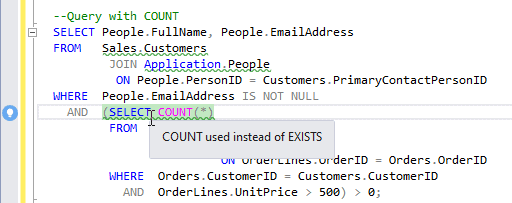
Figure 1: PE013 warning in SQL Prompt
Of course, as a diligent programmer, I now test both, rather than rely on the wisdom of built-in rules, or something I read on the Internet.
For a task such as this, I suggest two quick tests to perform: compare your version of the query, and the viable alternatives, in terms of their execution statistics and then, if necessary, their execution plans. Note that, the more realistic the data set you are using the more obvious differences may appear.
Query execution statistics
The simplest way to view the timings and other execution statistics for individual queries is to use STATISTICS IO/TIME, as follows (although STATISTICS IO introduces significant overhead in some cases, and you may prefer to use Extended Events).
|
1 2 3 4 5 6 |
SET STATISTICS IO, TIME ON; --turn on io and time stats --clear the procedure cache for the WideWorldImporters DB ALTER DATABASE SCOPED CONFIGURATION CLEAR PROCEDURE_CACHE; -- Query with EXISTS -- Query with COUNT(*) -- Query with DISTINCT |
Execute each query a few times to get the statistics related only to executing the plan (not compiling it or caching data to memory). I also advise running each of the statements individually or some overhead in the query execution process may be added or lost from the time statistics.
I won’t reel off the statistics here but I saw no significant difference in elapsed time for any of the query variations, and for the COUNT and EXISTS queries, the execution statistics, including logical reads (from memory) and physical reads (from disk) were identical.
In more interesting cases, you might find that a less readable solution uses less CPU, less I/O (memory and disk), and takes less time. The question then becomes: is it so much less time that implementing a more cryptic way to answer the question might be worth it? This decision is not always simple. If a query runs a million times a day, saving a few milliseconds is worth it. If it runs once per day, then saving 10 seconds is almost certainly not worth it, especially if it means no one else can understand how the code works.
In this case, it’s worth considering briefly why there was no performance difference between COUNT and EXISTS. This might seem surprising because, logically, it is easy to explain why the EXISTS solution might be faster, since it stops looking for matching orders for a customer as soon as it finds the first one. The COUNT solution, and the others, as written, process all the order lines for every person who has made a purchase, then reject those that don’t meet the “greater than no orders” criteria for purchases over 500.
The execution plans reveal the answer.
Execution plans
Note that WideWorldImporters includes the FilterCustomersBySalesTerritoryRole security policy that I temporarily disabled so that it didn’t complicate the plans; only ever do this in development!
|
1 |
ALTER SECURITY POLICY Application.FilterCustomersBySalesTerritoryRole WITH (STATE = OFF); |
In my tests the execution plans for the COUNT and EXISTS queries were the same, as shown in Figure 2.
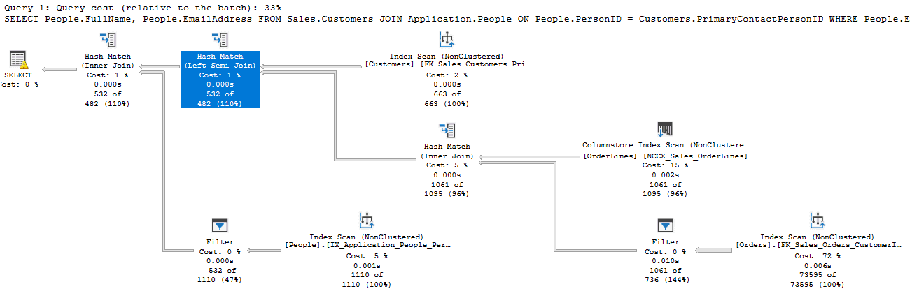
Figure 2: The query plan for the COUNT(*) and EXISTS variants of the query
In almost every query example, you will likely find that the EXISTS and the COUNT queries have the same plan. Although logically the former is more efficient, in fact the query optimizer can often rewrite a query to a mathematically equivalent version that performs better, and in fact, it treats these two variants in the same way whenever it can, so the plans, and performance, are the same. Phil Factor reported similar findings in his PE019 article on the use of EXISTS instead of IN.
However, as complexity increases in a query, the optimizer may not always be able to work its magic, so you may still see some cases where the COUNT variant really is slower, as well as less readable. That said, I tested more complex versions of these queries (though still with the same predicate condition) on tables up to several hundred gigabytes in size, and still saw no differences.
However, I did find small differences if I changed the predicate condition to “greater than or equal to zero“. For example, for the COUNT(*) query:
|
1 |
........AND OrderLines.UnitPrice > 500) >= 0; |
Mathematically, this query must return data. Yet, the plan for the COUNT query includes a few extra operators; a Hash Match (Aggregate) operator, to compute the COUNT(*) value, a Compute Scalar, and a Filter to filter out the rows where the COUNT(*) = 0. Collectively, they accounted for less than 2% of the work of this query.
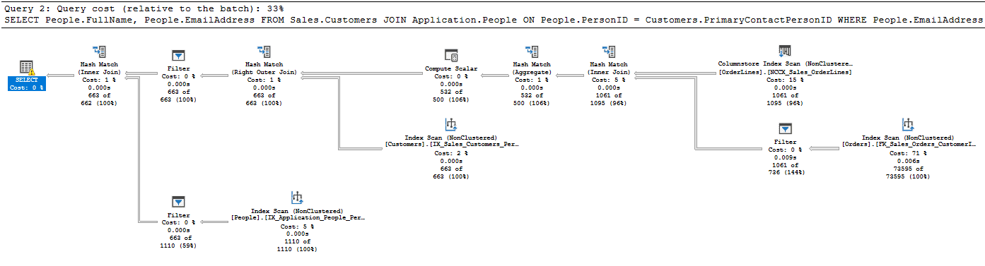
Figure 3: The query plan for the COUNT(*)>= query
Finally, I won’t show it here, but the plan for the DISTINCT query shows it to be a slightly higher costing implementation at 34% of the expected costs, to 33% each for the other two. The extra costs in the DISTINCT version of the query are mainly that it needs a Sort to implement the Distinct operator to remove duplicate values.
Whereas the previous queries use a semi-join between Customers and Orders (a semi-join is implemented as a correlated subquery, where you essentially join to the tables, but do not return any rows from one input, Orders table in this case), here we get a JOIN that will add the data to the set during processing resulting in slightly larger memory use. The resulting difference in performance is negligible, still, but this method is likely not to scale as well to large data volumes.
Considerations and false positives for code analysis rules
One of the interesting things with code analysis is that if I write the query as follows, using a variable for the COUNT filter, the results will be correct, I don’t see the PE013 warning, but I do get the poorer plan (the one in Figure 3).
|
1 2 3 4 5 6 7 8 9 10 11 12 |
DECLARE @countvalue int = 0; SELECT People.FullName, People.EmailAddress FROM Sales.Customers JOIN Application.People ON People.PersonID = Customers.PrimaryContactPersonID WHERE People.EmailAddress IS NOT NULL AND (SELECT COUNT(1) FROM Sales.Orders JOIN Sales.OrderLines ON OrderLines.OrderID = Orders.OrderID WHERE Orders.CustomerID = Customers.CustomerID AND OrderLines.UnitPrice >= 500) > @countvalue; |
Obviously, if the value of @countvalue is always set to a literal value, this is not an ideal way to write the query, introducing what looks like a variable value to the optimizer, causing it to pick a plan that allows for a different value for @countvalue (especially if you are using this just to avoid the code analysis warning to make your team code review easier).
If the value for @countvalue is a parameter allowing the query to do more than simple or existence of a row, then this technique is the best way to provide the answer to the questions like “give me the emails of all customers who have ordered 2 or more items of unit price greater than 500” by setting the @countvalue variable to 2. And then asking for 5 or more is a simple change of a parameter.
If you’re wondering if using COUNT(1), instead of COUNT(*) makes any difference to performance: it makes no difference what the scalar expression is, unless it includes a column in the expression that could cause it to evaluate to NULL. The scalar value without a column reference is not evaluated, even if it is nonsense like 1/0:
|
1 |
SELECT COUNT(1/0) FROM Sales.Orders; |
This returns 73595, not Divide-By-Zero as you would expect. Any scalar expression will be ignored and counted.
Finally, note that the static code analysis bases the rule on the 0 in the magnitude Boolean expression. Ending the COUNT(*) query with any of the following will cause the same alert, even though they have very different meanings, and are hence false positives to the rule, though none of the following examples are the ideal solution to the problem.
|
1 2 3 4 5 6 7 8 9 |
--First two are equivalent to NOT EXISTS AND OrderLines.UnitPrice >= 500) = 0; AND OrderLines.UnitPrice >= 500) <= 0; --Nonsense, COUNT cannot be < 0 AND OrderLines.UnitPrice >= 500) < 0; --Equivalent to EXISTS AND OrderLines.UnitPrice >= 500) > 0; --Will always be true AND OrderLines.UnitPrice >= 500) >= 0; |
Summary
There are always many ways to solve a problem, and in all cases, it is best to look for the simplest solution. Simplicity, naturally, gets harder to achieve the more complex the problem you’re trying to solve. Nevertheless, I always suggest you start with the query that makes the most sense and work from there.
For finding correlated rows based in criteria that at least one row must exist, it’s clear that using EXISTS is the most appropriate solution. It is readable, answers the question in a direct and simple fashion, and will perform as least equivalently to any alternative solution. While I wasn’t able to detect any performance advantage to using EXISTS over COUNT, the readability factor is enough to warrant taking code analysis rule PE013 seriously, for the sake of your future self, and other programmers.
Tools in this post
You may also like
-

Article
How to record T-SQL execution times using a SQL Prompt snippet
Phil Factor shares a SQL Prompt snippet called timings, which he uses as a standard testbed for getting execution times for procedures and functions.
-

Article
Quick SQL Prompt tip – script objects as ALTER in two clicks
Working in a large database can be difficult at times. While many of us might learn the meanings and definitions of most objects, it’s easy to forget the exact ways in which some objects work, or what the behavior is in certain calls. This is one place where having tools that assist you like SQL
-
Article
When to use the SELECT…INTO statement (PE003)
SELECT…INTO is a useful shortcut for development work, especially for creating temporary tables. However, it no longer has a clear performance advantage and should be avoided in production code. It is better to use a CREATE TABLE statement, where you can specify constraints and datatypes in advance, making it less likely that inconsistencies will sneak into the data.
-
Article
SQL Prompt Snippets to Drop Columns and Tables and Handle Associated Dependencies
Louis Davidson provides a pair of SQL Prompt snippets that will help you deal with dependencies, whenever you need to drop columns or tables.
-
Article
SQL Prompt Safety Net Features for SSMS: SQL History
Mistakes occasionally happen. Sometimes you accidentally close an SSMS query tab without saving it, before realizing it contained an essential bit of code. Occasionally, you make some ill-judged 'refinements' to working code and now just wish you could rewind your tab back in time an hour and forget the whole sorry episode. Now and again, SSMS just conspires against you and crashes unexpectedly, and you lose all your currently open query tabs, some of which you hadn't saved. SQL History offers a useful safety net in the event of any of these unfortunate events.


