Edward Pollack in T-SQL Programming Demystifying PIVOT and UNPIVOT in T-SQL Learn how to use T-SQL PIVOT and UNPIVOT operators with clear examples — from basic row-to-column transforms to dynamic SQL... 20 May 2026 12 min read 4
Greg Low in SQL Server What are managed identities in SQL Server 2025? A complete guide Learn how managed identities in SQL Server 2025 enhance security by eliminating passwords and enabling seamless Microsoft Entra authentication for... 05 May 2026 6 min read 1
Ben Johnston in SQL Server A complete guide to Azure SQL Managed Instance server and database configuration options A tested reference of sp_configure, ALTER DATABASE, and tempdb options that aren't supported in Azure SQL Managed Instance -plus the... 13 May 2025 10 min read
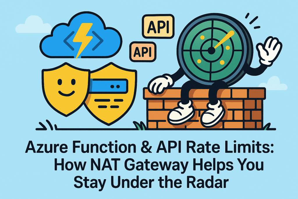
Dennes Torres in Blogs Azure Function & API Rate Limits: How NAT Gateway Helps You Stay Under the Radar Rate limit is common when consuming API’s: They control how many calls you can make in an interval of time.... 23 April 2025 4 min read 1
Ben Johnston in Databases 5 key problems from a SQL Server to Azure SQL Managed Instance migration (and how to avoid them) Planning an Azure SQL Managed Instance migration? Here are five surprises a real transactional SQL Server move uncovered - and... 31 March 2025 10 min read 2
Dennes Torres in Blogs Azure SQL Serverless: Discover What’s new and Increase Your Savings Before jumping into the news and code, let’s start from the beginning: Why does someone use Azure SQL Serverless? The... 22 January 2025 3 min read 21
Koen Verbeeck in Azure How To Embed Your Azure Logic Apps in a Metadata-driven Data Platform In this article, I am going to explain how you can dial your productivity up to 11 when you’re dealing... 22 October 2024 27 min read
Koen Verbeeck in Azure How To Use Managed Identities in your Azure Logic Apps Azure Logic Apps are a cloud-based service where you can create low code workflows to automate your business processes or... 18 September 2024 10 min read
Blogs Louis Davidson in Blogs Creating an Azure PostgreSQL cluster and connecting to it One of the technologies that my new job brought with it was learning about all the various database platforms that... 04 November 2023 7 min read
Dennes Torres in Azure Microsoft Fabric: Lakehouse and Data Factory in Power BI environment Microsoft is merging Data Factory and Power BI Dataflows in one single ETL solution. It’s not a simple merging, but... 06 September 2023 12 min read
Dennes Torres in Blogs Microsoft Fabric: Data Warehouse Ingestion using T-SQL and more .In this blog I will illustrate how we can ingest data from a blob storage to a Microsoft Fabric Data... 24 May 2023 5 min read
Dennes Torres in Azure Data Intelligence on light speed: Microsoft Fabric This article is based on exciting information just released at Microsoft’s Build conference on May 23, 2023. What we have... 24 May 2023 11 min read
Azure Dennes Torres in Azure Azure Function and User Assigned Managed Identities Let’s talk about authentication between Azure Functions and resources used by Azure Functions and conclude with many poorly documented secrets... 03 January 2023 16 min read
BI Dennes Torres in BI How to automate table level refresh in Power BI You can automate Power BI table refreshes using PowerShell, an Automation Account, and Runbook. Dennes Torres explains how in this... 18 April 2022 14 min read
Azure Dennes Torres in Azure Eight Azure SQL configurations you may have missed Azure SQL Database has been around for over ten years and is constantly evolving with new capabilities and options. Dennes... 07 February 2022 12 min read
Azure Mike Wood in Azure Azure Policies and Management Groups You can define policies for your Azure SQL Databases for security and meeting your organization’s standards. Management groups simplify policies... 13 December 2021 11 min read
T-SQL Programming Dennes Torres in T-SQL Programming Azure Synapse Serverless SQL: Querying Blob Storage with OPENROWSET – Filepath Filtering, Partitioning, Parquet vs CSV, and External Tables Performance-tuning SQL queries against Azure Blob Storage using Synapse Serverless SQL pool - filepath filtering with the filepath() function, partition-based... 21 October 2021 18 min read
Azure Robert Sheldon in Azure The Azure SQL portfolio Microsoft provides many ways to run SQL Server in Azure, but which do you choose? In this article, Robert Sheldon... 01 September 2021 14 min read
Azure Dennes Torres in Azure How to query private blob storage with SQL and Azure Synapse Azure storage can be marked Private to control access. Dennes Torres explains how to query private blob storage with SQL... 21 July 2021 17 min read
Editorials Kathi Kellenberger in Editorials How to learn about Azure SQL It was always important to me to keep up with the latest versions of SQL Server, but especially so when... 09 July 2021 3 min read