Microsoft is merging Data Factory and Power BI Dataflows in one single ETL solution. It’s not a simple merging, but still these ETL tools are easier to use then ever.

In this article, I will demonstrate how to create a lakehouse and ingest data using a step-by-step walkthrough that you can follow along with. You will see that it is not very difficult and what features are available.

If you need a refresher on what Microsoft Fabric is, you can read the first article I wrote here overview of Microsoft Fabric and this other one to enable a free preview so you can try it out without spending money.

Creating the Lakehouse

Let’s create a new lakehouse, step by step.

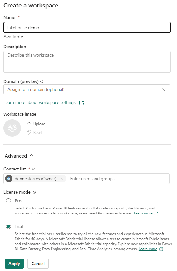
• Create a new workspace, let’s call it lakehouse demo. Use the trial resources explained here

 

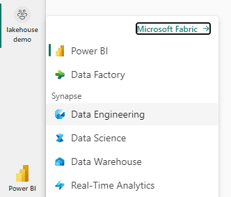
• Select the Data Engineering Experience

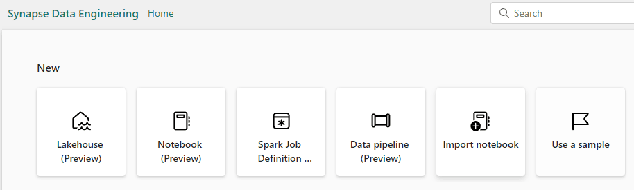
Synapse is present everywhere. The title of the window appears as Synapse Data Engineering

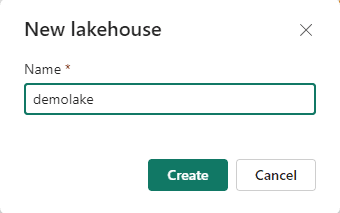
• Click the Lakehouse button and give it a name, demolake (or whatever you want to, but in the article it will be named demolake)

Ingesting Files into the Lakehouse

After creating the lakehouse, it’s time to create a data factory pipeline to ingest the data.

• Click the menu Get Data -> New Data Pipeline

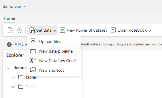
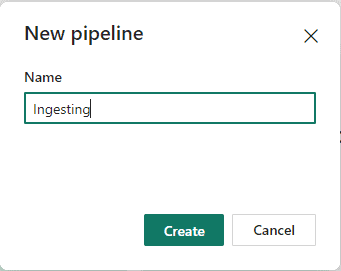
• Give a name to the pipeline as Ingesting

The wizard for data ingestion is one of the new features. It makes the work much easier than in previous iterations of these tools. The next image shows the first window of the wizard.

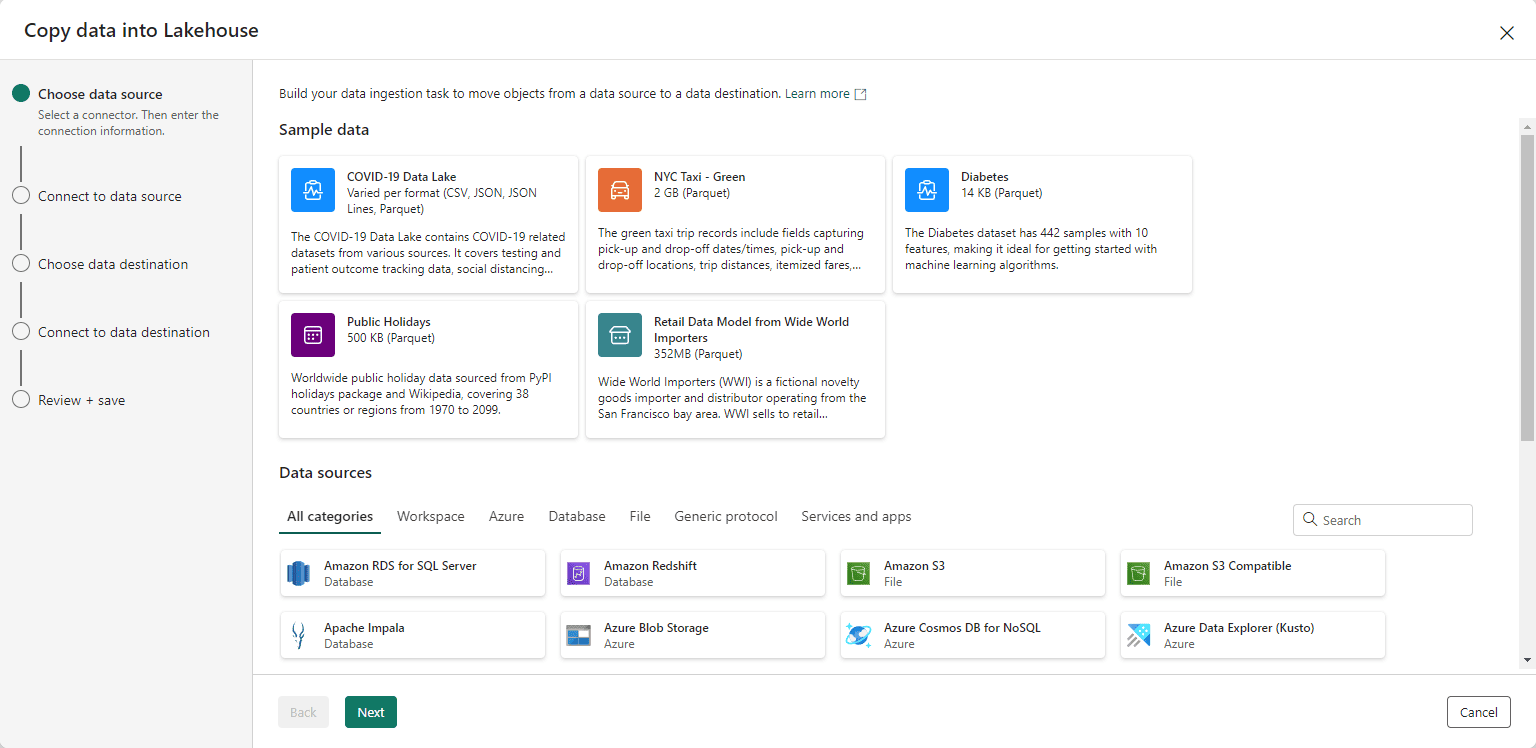
We will load information from a sample azure blob storage provided by Microsoft and with anonymous access.

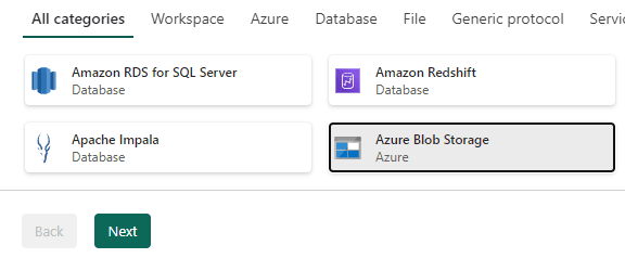
• Select Azure Blob Storage as the source and click the Next button.

On the following screen, you can choose between an existing connection or a new one. The Power BI environment saves connections to be reused by different objects and this includes Microsoft Fabric objects. You can read more about Power BI and Fabric connection management

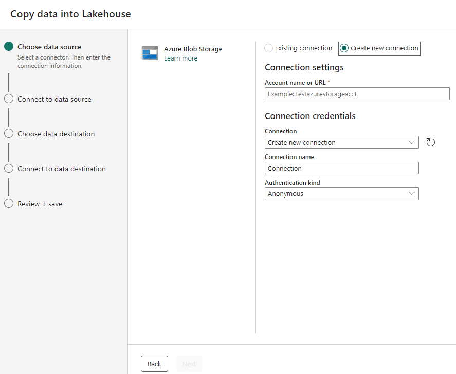
• On the Account Name or URL textbox, type the following address: https://azuresynapsestorage.blob.core.windows.net/sampledata
• On the Connection Name textbox, type wwisample
• Click the Next button.

Here we can find how easy a wizard can be: After noticing we don’t have anonymous access direct to the container, the wizard gives us another window to type the precise path we would like to access and get the data from:

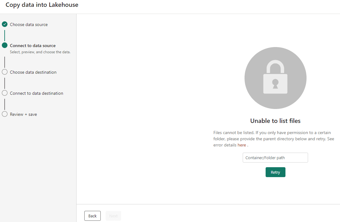
• On the textbox in the middle of the wizard, type the following path: /sampledata/WideWorldImportersDW/parquet
• Click the Retry button

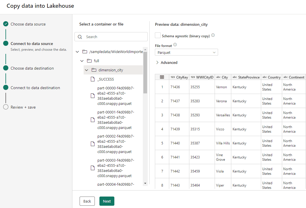
After the retry, we will be able to see the list of folders available for us and the options about the format for ingestion.

• Select the folder full
• Mark the checkbox Schema agnostic (binary copy)

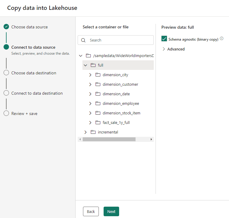
The binary copy option, like the one existing in Data Factory’s Copy Activity, allow us to copy not only multiple files but multiple folders to the Files area of the lakehouse.

The same couldn’t be done to the Tables area of the lakehouse, we would need to import the tables one by one with the correct schema.

• Click the Next button.
• Choose the option Existing Lakehouse

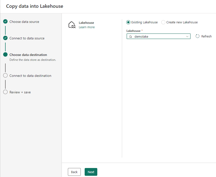
Choosing the lakehouse is the first option on the destination choice.

• Click the Next button

We need to select the destination of the files being copied. The Tables destination is disabled because we selected the binary copy.

The Browse button allow you to organize the files you are copying according to your folder structure. In our example, we don’t have a folder structure yet, so we don’t need to click the Browse button.

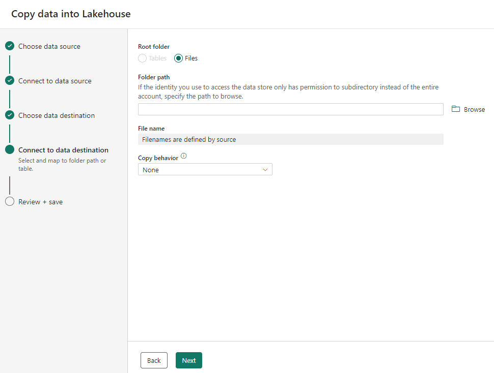
• Click the Next button

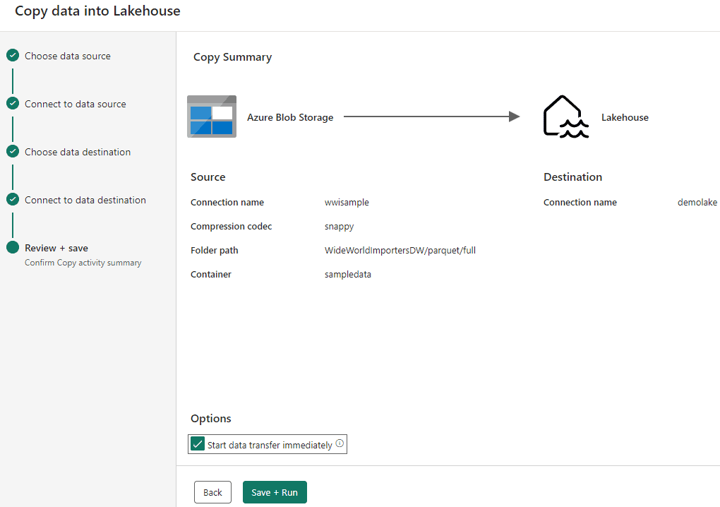
At this point, all the configuration needed for the ingestion is done. We only need to conclude the Wizard and ask for the execution.

• Mark the checkbox Start data transfer immediately.
• Click the Save + Run button.

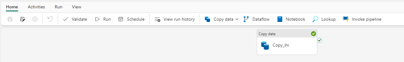
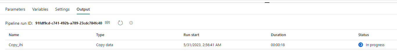
The pipeline will be executed, and you may notice it’s a simple Copy Activity, which is usual for a Data Factory Pipeline. As explained, the pipelines and dataflows in Microsoft Fabric are a merge between Power BI and Data Factory features.

• Click the demolake button on the left bar.

The left bar adapts itself with icons of recently opened resources, allowing you to navigate among them.

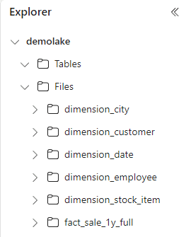
On the lake explorer, you will notice the folders for each table inside the Files area. The shows you that the data is ingested.

Ingest as Table

We ingested the data as binary files. Let’s analyse how would it be to ingest the data as a Table.

Back to selecting the source, during the Copy Data into Lakehouse wizard, if we select one single folder, which contains one single table, and select the correct data format, we can ingest the information to the Table area of the lakehouse.

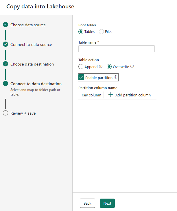
When selecting tables as destination, we can select the following options:

• The table name
• The Action: We can Append the data to an existing table or overwrite the data of an existing table.
• Partitioning: All the storage is kept in Delta format. This format allows to partition the data according to field values. The partitioning will be done breaking the data in different folder. For example, if you choose to partition by Year, a different folder will be created for each year.

Files and Tables

The Files area in the lakehouse is dedicated to RAW data, the data just ingested. After the ingestion, we should load the data in the Tables area. The Tables area allow the following:

• The data will be specially optimized, being able to reach a performance up to 10x the regular delta table performance.
• The data is still 100% compatible with delta format.
• The data is available for SQL Queries using the SQL Endpoint

Even if the data in the Files area is already in Delta format, the tables will only be available for the SQL Endpoint if converted to the Tables area.

There are two different methods to convert the data form the Files area to the Tables area: We can use the UI or we can use a spark notebook.

Missing Point

In tools such as Synapse Serverless, we can use SQL to access data from storage in many different formats using the OPENROWSET function. However, this feature is not available in Microsoft Fabric, at least yet.

Converting the Files into Tables

Let’s analyse some differences in relation to the usage of the UI and the usage of a spark notebook:

UI Conversion	Spark Notebook
No writing options configuration	Custom writing options configuration
No partitioning configuration	Custom partitioning configuration
Manual Process	Schedulable process

The process of conversion is very simple:

• Right-Click the folder containing the files.
• Select Load To Tables -> New Table

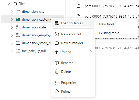
The Existing Table option allow us to add more data in an existing table manually. However, the process will be too manual, it would be better to schedule a notebook for this.

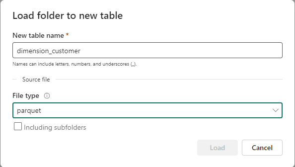
• On the Load new folder to table window, type the name of the table in the New table name textbox
• On the File type drop down, select parquet

• Repeat the steps 21-24 for each table
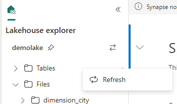
• On the lakehouse explorer, right click Tables and click Refresh.

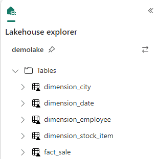
• The tables are now available in the Tables area.

• On the left bar, click the demolake button.

Let’s look on the storage behind the tables in the lakehouse.

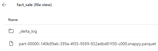
• Right click the fact_sale table
• On the context menu, click View files menu item.

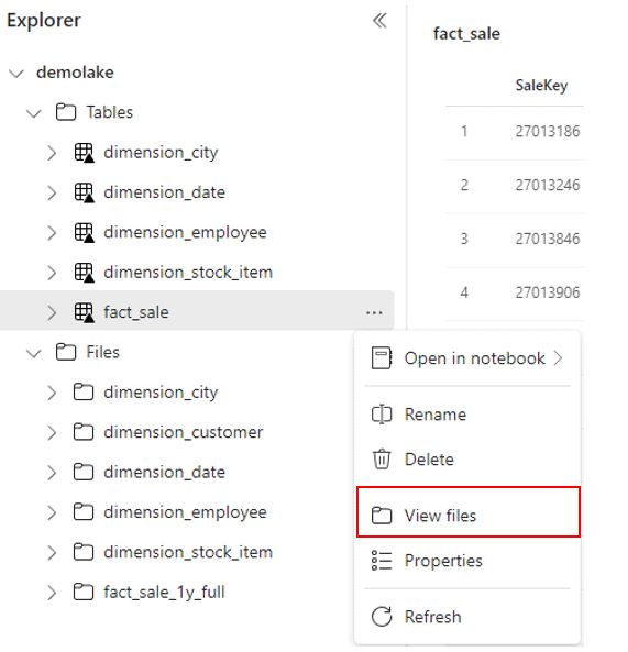
Mind how the files are stored in delta format.

Using a SQL Endpoint

The lakehouse provides a SQL Endpoint which allow us to use SQL language over the data.

Let’s make some experiments with the SQL Endpoint. We can use the box on the top right of the window to change the view from the lakehouse to the SQL Endpoint.

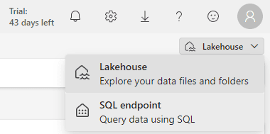
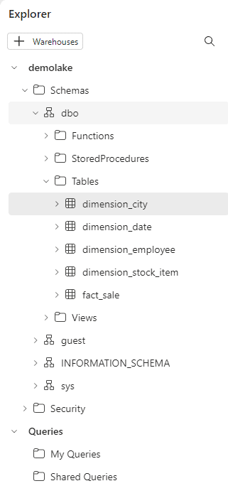
The SQL Endpoint changes the Explorer view to a database format, showing only the Tables content as a database.

On this view, we have the option to create queries, either SQL Queries or Visual Queries. The capability to create queries is available in many different places in Power BI and Microsoft Fabric environment:

Power BI Datamarts

I wrote about them and query creation here (https://www.red-gate.com/simple-talk/databases/sql-server/bi-sql-server/datamarts-and-exploratory-analysis-using-power-bi/) when the UI was still Design Tab and SQL Tab. The UI is slightly different today, but the meaning is the same – query creation, with two types of queries.

Fabric Data Warehouse

I wrote about it here (https://www.red-gate.com/simple-talk/blogs/microsoft-fabric-data-warehouse-ingestion-using-t-sql-and-more/) at that point, I only wrote about using the SQL Queries to execute DDL statements.

This is, in fact, one of the differences between a Data Warehouse and a SQL Endpoint: The Data Warehouse has full DDL support, while the SQL Endpoint has limited DLL support.

Fabric Lakehouse

This is the example illustrated on this article.

Am I missing other places where the same UI was implemented? Probably. Add on the comments, please.

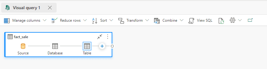
Creating a Visual Query

• Click the New Visual Query button.
• Drag the Fact_Sale table to the Visual Query area.

• Drag the Dimension_Customer table to the Visual Query area.

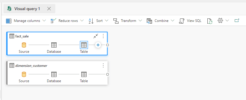
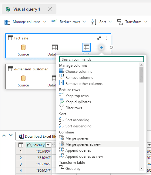
• Click the ‘+’ button on Fact_Sale in the Visual Query area and select Merge queries as new

• Select the Dimension_Customer table on the Right table for merge drop down.

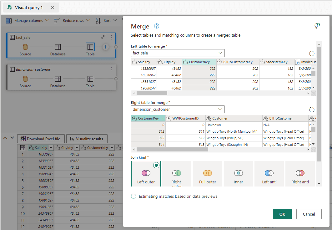
• Click the Ok button.
• Click on the Data Display area and move the focus to the last column on the right.

   

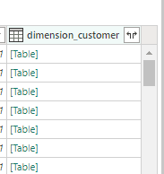
• Click the Expand button and select only the BuyingGroup column.

   

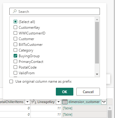
After making a join between the tables, the columns from the first table are kept and we choose which columns from the second table we would like to include in the join as well.

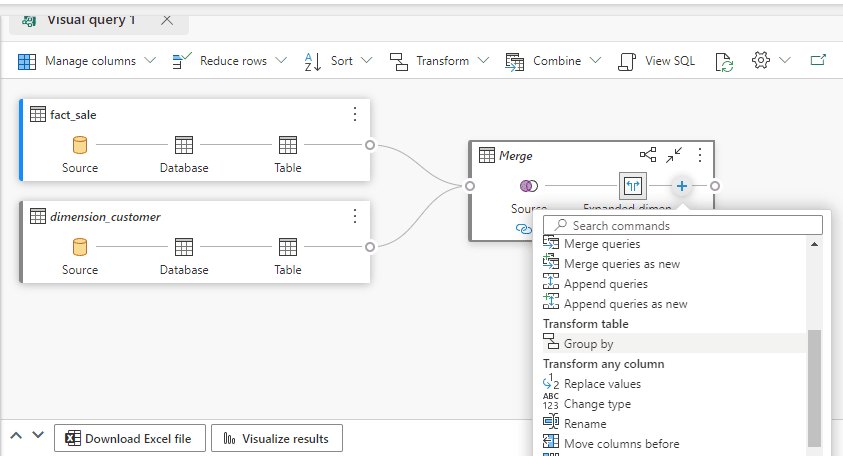
• Click the ‘+’ button on the merged table and select Group By

   

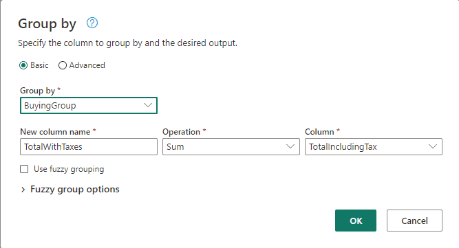
• On the Group By window, Select BuyingGroup field in the Group By dropdown.
• On the New column name textbox type TotalWithTaxes
• On the Operation dropdown, select Sum.
• On Column dropdown, select TotalIncludingTax field.

We have only used the Basic option on this example. The Advanced option would allow us to add multiple grouping fields and multiple aggregations.

• Click the Ok button.

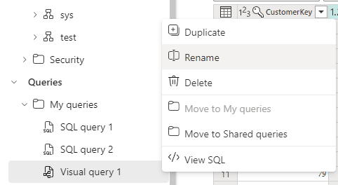
• On the left window, under My Queries, click the expand “..” button close the Visual Query 1 and select Rename.

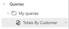
• On the Rename window, on the Name textbox, type Totals By Customer

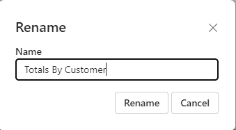
• Click the Rename button.

  

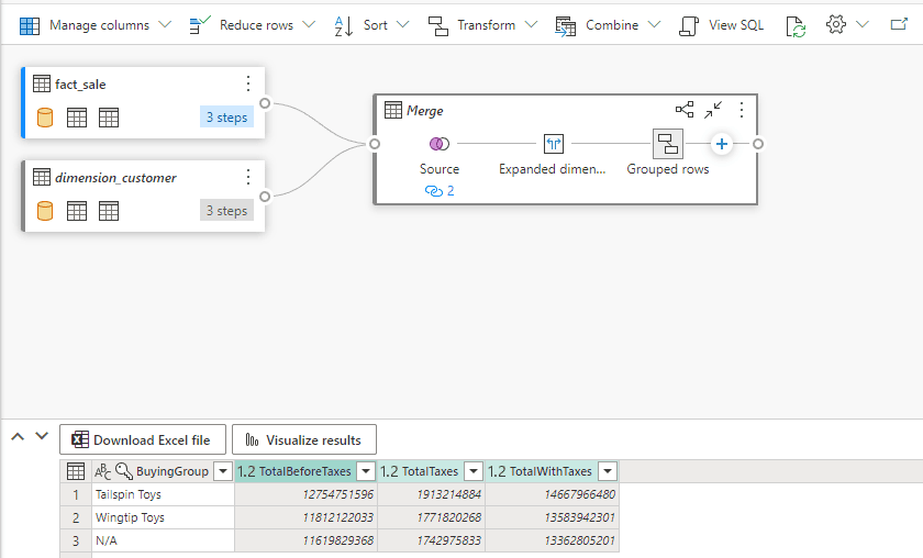
What to do with the queries

After creating a visual query, we can use it in many ways:

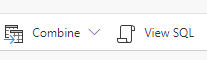
• We can click the View SQL button and use the SQL to create a view or a materialized object.

At the time of publishing this article, the preview version has a bug and only shows the initial SQL query, not the final query with all the transformations. We hope this is fixed soon.

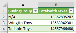
• We can download an excel file and continue our exploration on the Excel file.

The Excel is dynamically configured to execute the query against the Lakehouse. As a result, the data is dynamically load from the lake every time we open the Excel. We can save this file and use it to analyse the same query as many times as we would like.

These are the steps to download and use an Excel file:

1. Click the Download Excel File button on the Display area.

• Open the downloaded excel file.
• Click the Enable Editing button.

This first warning is caused because the Excel file was downloaded from the web. This is the first level of security.

• On the Security Warning, click Enable Content button.

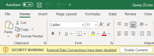
The Excel file opened contains dynamic content, including a SQL query to build an Excel table. This is active content which needs to be enabled. This is the 2nd level of security.

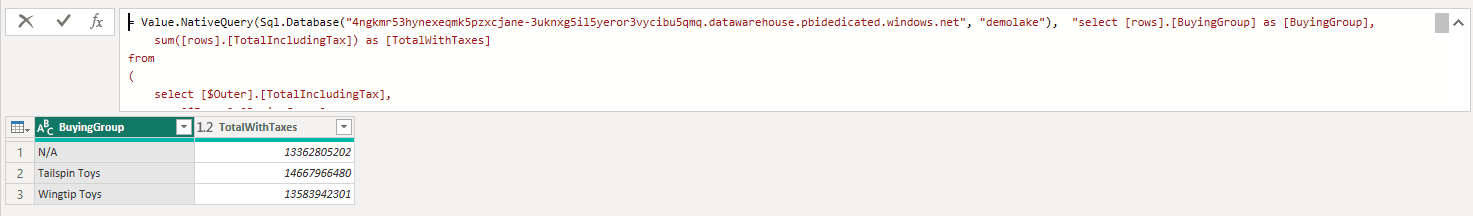
• On the Native Database Query window, click the Run button.

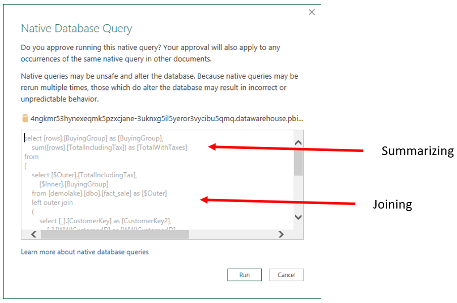
We will be running a SQL query pointing to a server. Excel shows the query and asks for confirmation. This is the 3rd level of security.

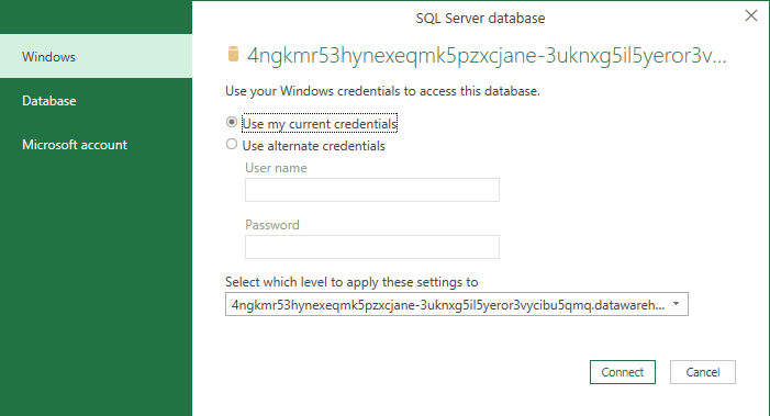
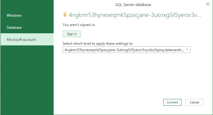
• On the SQL Server Database window, choose Microsoft Account on the left side.

• Click the Sign In button and login with your Microsoft Fabric account.

Mind the SQL Server address on this window: It’s in fact the SQL Endpoint address from the lakehouse.

• Click the Connect button.

The SQL query will only be executed if the user opening the Excel file has permissions on the Microsoft Fabric SQL Endpoint. This is the 4th level of security.

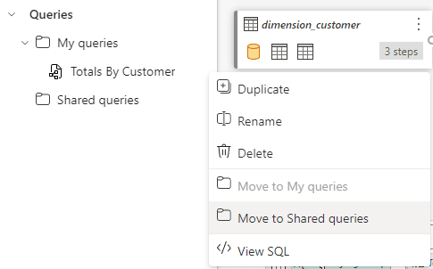
• We can turn the query into a shared query and allow other team members to continue the data exploration.

On the context menu for the query, we choose Move to Shared Queries. We can move back to My Queries if we would like so.

There are only these two options: Or the query is private to the user, or it’s accessible to every user who has access to the lakehouse.

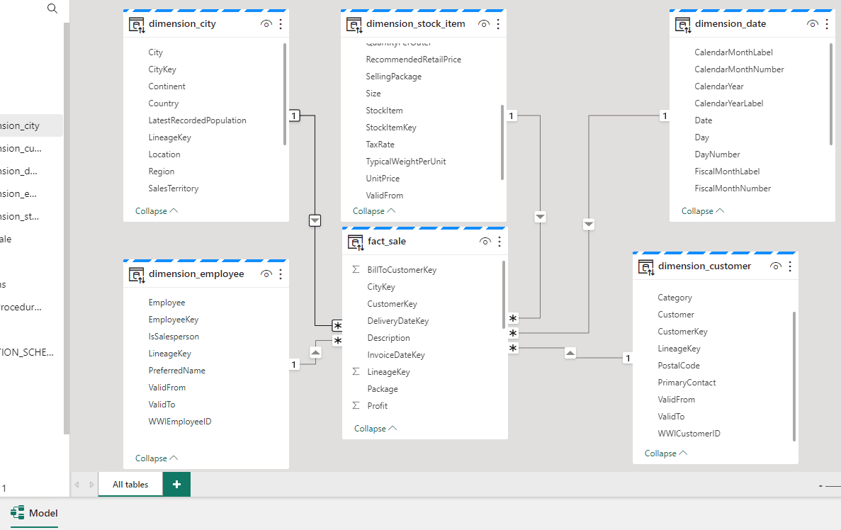
Modelling the Tables

The SQL Endpoint in a lakehouse allow us to model the tables in the same way it does in a Data Warehouse and I illustrated on my article about Data Warehouse.

In the same way, the model is stored in the default dataset. By doing so, we establish a default modelling we would like the consumers to have when accessing the lakehouse. This is not only about table relationships, but also the creation of measures.

Creating a Report

I already explained the process of building a report on my article about Data Warehouse, it’s very similar. I will approach details about the access from Power BI to OneLake in future articles.

The only difference worth mentioning on this point is that clicking on the button Visualize Results will create a dataset and a report from the query we visually generated. We can download and inspect the resulting dataset. It’s built with a single SQL query towards the lakehouse SQL Endpoint.

Summary

Microsoft Fabric is a great tool, as I highlighted on my overview. It provides plenty of options about how to manage our data, either using a Data Warehouse, explained in a previous article, or a lake house, explained on this article. All the options linked by a common environment, the Power BI, going way beyond the BI area.

In future articles I will approach how to choose the option to use and how to organize these scenarios on an enterprise level.