
SQL Server graph databases (introduced in SQL Server 2017) model complex many-to-many and hierarchical relationships using node tables (entities) and edge tables (relationships). You create graph tables with CREATE TABLE…AS NODE and CREATE TABLE…AS EDGE, then query them using the MATCH clause, which traverses relationships without complex self-joins or recursive CTEs.
Graph databases are built on top of the standard SQL Server engine – you use the same tools (SSMS), the same T-SQL, and the same transactions, but with native support for relationship-heavy data like social networks, recommendation engines, and organizational hierarchies.
The series so far:
- SQL Server Graph Databases - Part 1: Introduction
- SQL Server Graph Databases - Part 2: Querying Data in a Graph Database
- SQL Server Graph Databases - Part 3: Modifying Data in a Graph Database
- SQL Server Graph Databases - Part 4: Working with hierarchical data in a graph database
- SQL Server Graph Databases - Part 5: Importing Relational Data into a Graph Database
With the release of SQL Server 2017, Microsoft added support for graph databases to better handle data sets that contain complex entity relationships, such as the type of data generated by a social media site, where you can have a mix of many-to-many relationships that change frequently. Graph databases use the same table structures found in traditional SQL Server databases and support the same tools and T-SQL statements, but they also include features for storing and navigating complex relationships.
This article is the first in a series about SQL Server graph databases. The article introduces you to basic graph concepts and demonstrates how to create and populate graph tables, using SQL Server Management Studio (SSMS) and a local instance of SQL Server 2017. In the articles to follow, we’ll dig into how to query a graph database and modify its data, but for this article, we’re starting with the basics.
The SQL Server Graph Database
SQL Server’s graph databases can help simplify the process of modeling data that contains complex many-to-many and hierarchical relationships. At its most basic, a graph database is a collection of nodes and edges that work together to define various types of relationships. A node is an entity such as a person or location. An edge is a relationship between two entities. For example, a relationship might exist between a location such as Toledo and a person named Chris, who lives in Toledo. Chris and Toledo are the entities, and ‘lives in’ is the relationship between the two.
A node table in SQL Server is a collection of similar entities, and an edge table is a collection of similar relationships. To help understand how this works, consider the graph model shown in the following figure, which is based on a fictitious fish-lovers forum. The model includes three nodes (FishSpecies, FishLover, and FishPost) and three edges (Likes, Posts, and LinksTo).
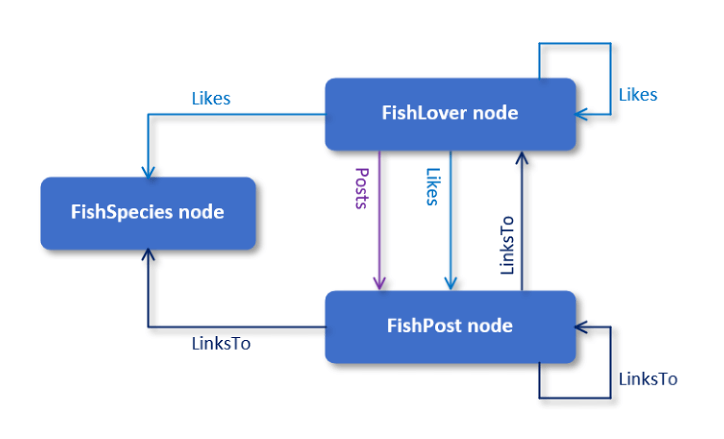
The rectangles represent the nodes, and the arrows connecting the nodes represent the edges, with the arrows pointing in the direction of the relationship. For example, the Likes edges can define any of the following relationships:
- A fish lover likes a fish species.
- A fish lover likes a post about fish.
- A fish lover likes another fish lover.
You can represent all three relationships as data in a single edge table in the graph database, with each relationship in its own row. A node table works much the same way, except that it includes a row for each entity. You can also associate properties with both nodes and edges. A property is a key-value attribute that is defined as a column in a node or edge table. For example, the FishSpecies node might include properties for storing the common and scientific names of each species. The properties are created as user-defined columns in the FishSpecies table. When creating a node table, you must include at least one property.
For most operations, node and edge tables work just like any other SQL Server user-defined table. Although there are a few limitations—such as not being able to declare temporary tables or table variables as node or edge tables—most of the time you’ll find that working with graph tables will be familiar territory.
Where things get a bit unclear is with the graph database itself. Although the name might suggest that you’re creating a new type of database object, that is not the case. A graph database is merely a logical construct defined within a user-defined database, which can support no more than one graph database. The existence of the graph database is relatively transparent from the outside and, for the most part, is not something you need to be concerned about. When working with graph databases, your primary focus will be on the graph tables and the data they contain.
In general, a graph database provides no capabilities that you cannot achieve by using traditional relational features. The promise of the graph database lies in being able to organize and query certain types of data more efficiently. Microsoft recommends that you consider implementing a graph database in the following circumstances:
- You need to analyze highly interconnected data and the relationships between that data.
- You’re supporting data with complex many-to-many relationships that are continuously evolving.
- You’re working with hierarchical data, while trying to navigate the limitations of the HierarchyID data type.
SQL Server’s graph database features are fully integrated into the database engine, leveraging such components as the query processor and storage engine. Because of this integration, you can use graph databases in conjunction with a wide range of components, including columnstore indexes, Machine Learning Services, SSMS, and various other features and tools.
Defining Graph Node Tables
To create a graph database based on the model shown in the preceding figure, you must create three node tables and three edge tables. Microsoft has updated the CREATE TABLE statement in SQL Server 2017 to include options for defining either table type. As already noted, you can create the tables in any user-defined databases. For the examples in this article, I created a basic database named FishGraph, as shown in the following T-SQL code:
|
1 2 3 4 5 6 |
USE master; GO DROP DATABASE IF EXISTS FishGraph; GO CREATE DATABASE FishGraph; GO |
As you can see, there’s nothing special going on here. You create the database just like any other user-defined database. There’s nothing special you need to do to set it up to support a graph database.
If you plan to try out these examples for yourself, you can use the FishGraph database or one of your own choosing. Whatever you decide, the next step is to create the FishSpecies node table, using the following CREATE TABLE statement:
|
1 2 3 4 5 6 7 8 9 |
USE FishGraph; GO DROP TABLE IF EXISTS FishSpecies; GO CREATE TABLE FishSpecies ( FishID INT IDENTITY PRIMARY KEY, CommonName NVARCHAR(100) NOT NULL, ScientificName NVARCHAR(100) NOT NULL ) AS NODE; |
The column definitions should be fairly straightforward. What’s important here is the AS NODE clause, which you must include to create a node table. When you specify this clause, the database engine adds two columns to the table (which we’ll get to shortly) and creates a unique, non-clustered index on one of those columns.
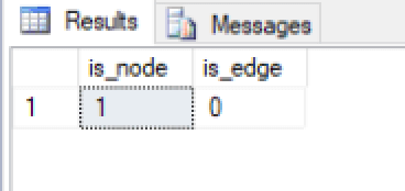
You can verify whether the table has been created as a node table by querying the sys.tables view. With the release of SQL Server 2017, Microsoft updated the view to include the is_node and is_edge bit columns. If the table is a node table, the is_node column value is set to 1, and the is_edge column value is set to 0. If an edge table, the values are reversed. The following example uses the view to confirm that the FishSpecies table has been defined correctly:
|
1 2 |
SELECT is_node, is_edge FROM sys.tables WHERE name = 'FishSpecies'; |
The SELECT statement returns the results shown in the following figure, which indicate that FishSpecies was created as a node table.
Microsoft also updated the sys.columns view to include the graph_type and graph_type_desc columns. You can use the view and new columns to learn more about the FishSpecies table:
|
1 2 3 |
SELECT name, graph_type, graph_type_desc FROM sys.columns WHERE object_id = OBJECT_ID('FishSpecies'); |
The following figure shows the columns created for the FishSpecies table.
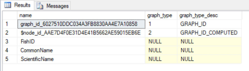
When you create a node table, the database engine adds the graph_id_<hex_string> and $node_id_<hex_string> columns and creates a unique, non-clustered index on the $node_id column. The database engine uses the first column for internal operations and makes the second column available for external access. The $node_id column stores a unique identifier for each entity, which you can view when querying the data. This is the only column of the two you need to be concerned with. In fact, if you were to query the table directly, you would see only the $node_id column, not the graph_id column.
The graph_type and graph_type_desc columns returned by the sys.columns view are specific to the auto-generated columns in a graph table. The columns indicate the types of columns that the database engine generated. The type is indicated by a predefined numerical value and its related description. Microsoft does not provide a great deal of specifics about these codes and descriptions, but you can find some details in the Microsoft document SQL Graph Architecture. Again, your primary concern is with the $node_id column and the data it contains.
After you’ve created your table, you can start adding data. Running an INSERT statement against a node table works just like any other table. You specify the target columns and their values, as shown in the following example:
|
1 2 3 4 5 6 7 8 9 10 11 |
INSERT INTO FishSpecies (CommonName, ScientificName) VALUES ('Atlantic halibut', 'Hippoglossus hippoglossus'), ('Chinook salmon', 'Oncorhynchus tshawytscha'), ('European seabass', 'Morone (Decentrarchus) labrax'), ('Gizzard shad', 'Dorosoma cepedianum'), ('Japanese striped knife jaw', 'Oplegnathus faciatus'), ('Northern pike', 'Esox lucius'), ('Pacific herring', 'Clupea pallasi'), ('Rainbow trout', 'Oncorhynchus mykiss'), ('Sole (Dover)', 'Solea solea'), ('White bass', 'Morone chrysops'); |
Of course, you can add whatever fish species you have a particular fondness for. My choices here were completely arbitrary. But if you do stick with my data and then query the FishSpecies table, your results should look similar to those in the following figure.
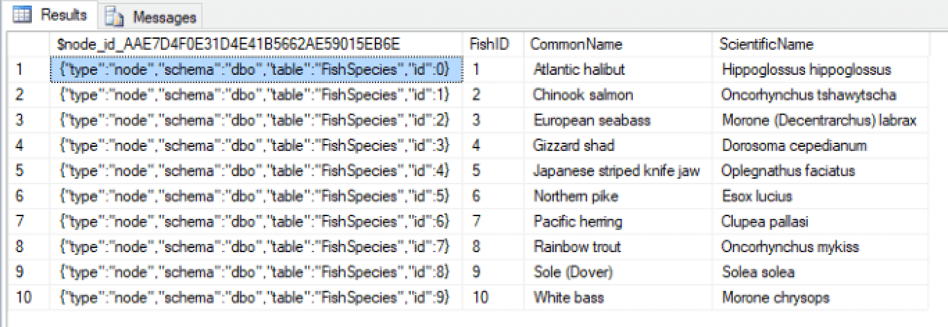
As mentioned above, the graph_id column does not show up in the results, but the $node_id column does, complete with auto-generated values. The database engine creates each value as a JSON string that provides the type (node or edge), schema, table, and a BIGINT value unique to each row. As expected, the database engine also returns the values in the user-defined columns, just like a typical relational table.
The next step is to create and populate the FishLover node table, using the following T-SQL code:
|
1 2 3 4 5 6 7 8 9 10 11 12 |
DROP TABLE IF EXISTS FishLover; GO CREATE TABLE FishLover ( FishLoverID INT IDENTITY PRIMARY KEY, Username NVARCHAR(50) NOT NULL, ) AS NODE; INSERT INTO FishLover (Username) VALUES ('powerangler'), ('jessie98'), ('hooked'), ('deepdive'), ('underwatercasey'); |
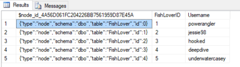
The table includes only two user-defined columns—FishLoverID and UserName—but you can define as many columns as necessary. For example, you might want to include first and last names, contact information, and other details, depending on the nature of the application. Once you’ve created the table, you can then run a query to verify the data. Your results should look similar to those shown in the following figure.
You can then take the same steps to create and populate the FishPost table, passing in whatever message text you wish:
|
1 2 3 4 5 6 7 8 9 10 11 12 13 |
DROP TABLE IF EXISTS FishPost; GO CREATE TABLE FishPost ( PostID INT IDENTITY PRIMARY KEY, Title NVARCHAR(50) NOT NULL, MessageText NVARCHAR(800) NOT NULL ) AS NODE; INSERT INTO FishPost (Title, MessageText) VALUES ('The one that got away', 'Lorem ipsum dolor sit amet, consectetuer adipiscing elit. Aenean commodo ligula eget dolor.'), ('A study in fish', 'Cum sociis natoque penatibus et magnis dis parturient montes, nascetur ridiculus mus.'), ('Hook, line and sinker ', 'Donec pede justo, fringilla vel, aliquet nec, vulputate eget, arcu.'), ('So many fish, so little time', 'Nullam dictum felis eu pede mollis pretium. Integer tincidunt.'), ('My favorite fish', 'Aenean leo ligula, porttitor eu, consequat vitae, eleifend ac, enim.'); |
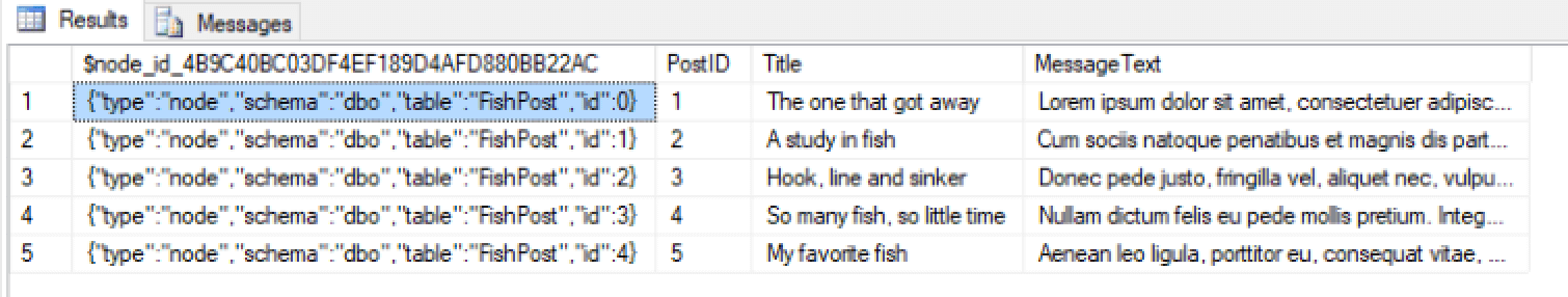
The following figure shows the results you would see if you stuck with the Lorem Ipsum data.
That’s all there is to creating and populating your node tables. Except for the AS NODE clause in the CREATE TABLE statement, most everything else is business as usual.
Defining Graph Edge Tables
Creating an edge table is similar to creating a node table except that you must specify the AS EDGE clause rather than the AS NODE clause. For example, to create the Posts table, you would use the following CREATE TABLE statement:
|
1 2 3 4 5 |
DROP TABLE IF EXISTS Posts; GO CREATE TABLE Posts ( ImportantFlag BIT NOT NULL DEFAULT 0 ) AS EDGE; |
The table definition is similar to a node table except that it does not include a primary key column (and, of course, it takes the AS EDGE clause). In this case, a primary key is not necessary, but if at some point you determine that you need a primary key, you certainly can add one. (You’ll see shortly why primary keys are useful for the node tables.)
Notice that the table definition also includes the ImportantFlag column. I included this primarily to demonstrate that you can add user-defined columns to your edge table, just like with node tables. That said, it’s not uncommon to create an edge table without user-defined columns, unlike a node table, which must include at least one user-defined column.
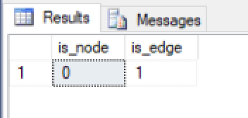
After creating the edge table, you can verify that it’s been defined correctly by querying the sys.tables view, as you saw earlier:
|
1 2 |
SELECT is_node, is_edge FROM sys.tables WHERE name = 'Posts'; |
If you did everything right, your results should look like those in the following figure.
You can also query the sys.tables view to verify column details, just like you did before:
|
1 2 3 |
SELECT name, graph_type, graph_type_desc FROM sys.columns WHERE object_id = OBJECT_ID('Posts'); |
The following figure shows the results returned on my system.
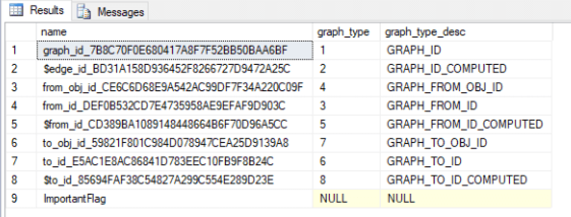
As you can see, the database engine adds eight columns to an edge table, rather than the two you saw with node tables. Again, refer to the SQL Graph Architecture document for descriptions of each column type. That majority of these columns are used by the database engine for internal operations. You need to be concerned primarily with the following three columns:
- The $edge_id_<hex_string> column uniquely identifies each relationship.
- The $from_id_<hex_string> column stores the $node_id value associated with the entity in the table where the relationship originates.
- The $to_id_<hex_string> column stores the $node_id value associated with the entity in the table where the relationship terminates.
As with the $node_id column in a node table, the database engine automatically generates values for $edge_id column. However, you must specifically add values to the $from_id and $to_id columns to define a relationship. To demonstrate how this works, we’ll start with a single record:
|
1 2 3 |
INSERT INTO Posts ($from_id, $to_id) VALUES ( (SELECT $node_id FROM FishLover WHERE FishLoverID = 1), (SELECT $node_id FROM FishPost WHERE PostID = 3)); |
The INSERT statement is defining a relationship in the Posts table between a FishLover entity whose FishLoverID value is 1 and a FishPost entity whose PostID value is 3. Notice that you can use the $node_id, $from_id, and $to_id aliases to reference the target columns, without having to come up with the hex strings.
To add data to the $from_id column, you must specify the $node_id value associated with the FishLover entity. One way to get this value is to include a subquery that targets the entity, using its primary key value. You can take the same approach for the $from_id column.
Inserting the data in this way demonstrates why it’s useful to add primary keys to the node tables, but not necessary for the edge tables. The primary keys on the node tables make it much easier to provide the $node_id value to the INSERT statement.
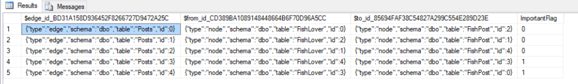
If you now query the Posts table, your results should look similar to those shown in the following figure.

The table should contain the new relationship, with the ImportantFlag set to 0, the default. You can now add a few more rows, using the following INSERT statements:
|
1 2 3 4 5 6 7 8 9 10 11 12 |
INSERT INTO Posts ($from_id, $to_id) VALUES ( (SELECT $node_id FROM FishLover WHERE FishLoverID = 3), (SELECT $node_id FROM FishPost WHERE PostID = 2)); INSERT INTO Posts ($from_id, $to_id) VALUES ( (SELECT $node_id FROM FishLover WHERE FishLoverID = 2), (SELECT $node_id FROM FishPost WHERE PostID = 5)); INSERT INTO Posts ($from_id, $to_id, ImportantFlag) VALUES ( (SELECT $node_id FROM FishLover WHERE FishLoverID = 5), (SELECT $node_id FROM FishPost WHERE PostID = 4), 1); INSERT INTO Posts ($from_id, $to_id, ImportantFlag) VALUES ( (SELECT $node_id FROM FishLover WHERE FishLoverID = 4), (SELECT $node_id FROM FishPost WHERE PostID = 1), 1); |
Notice that the last two INSERT statements also provide a value for the ImportantFlag column. When you query the Posts table, your results should now include all five rows.
The next step is to create and populate the Likes table, using the following T-SQL code:
|
1 2 3 4 5 6 7 8 9 10 11 12 |
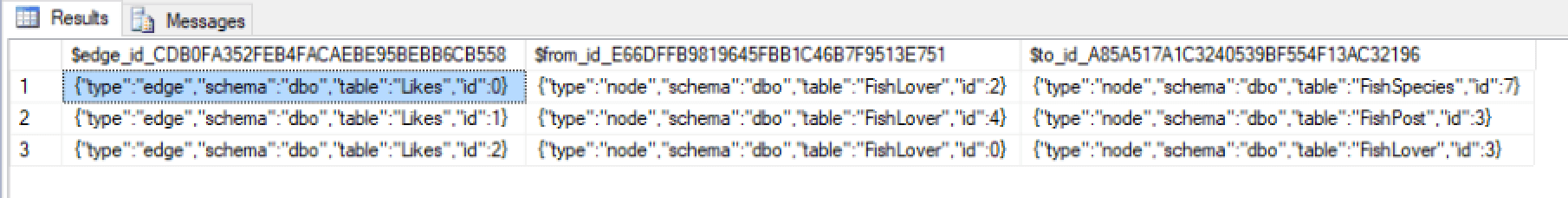
DROP TABLE IF EXISTS Likes; GO CREATE TABLE Likes AS EDGE; INSERT INTO Likes ($from_id, $to_id) VALUES ( (SELECT $node_id FROM FishLover WHERE FishLoverID = 3), (SELECT $node_id FROM FishSpecies WHERE FishID = 8)); INSERT INTO Likes ($from_id, $to_id) VALUES ( (SELECT $node_id FROM FishLover WHERE FishLoverID = 5), (SELECT $node_id FROM FishPost WHERE PostID = 4)); INSERT INTO Likes ($from_id, $to_id) VALUES ( (SELECT $node_id FROM FishLover WHERE FishLoverID = 1), (SELECT $node_id FROM FishLover WHERE FishLoverID = 4)); |
You can, of course, define any relationships you want. The important point to notice here is that you’re not limited to any one set of nodes. For example, the first INSERT statement creates a relationship between FishLover and FishSpecies, the second statement creates a relationship between FishLover and FishPost, and the third statement creates a relationship between FishLover and FishLover. This gives us the query results shown in the following figure.
You can take the same approach when creating and populating the LinksTo table:
|
1 2 3 4 5 6 7 8 9 10 11 12 |
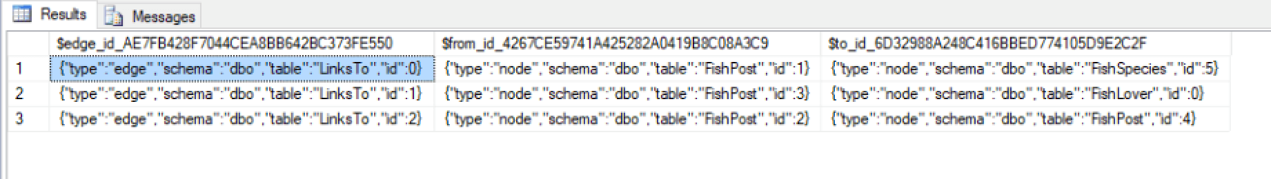
DROP TABLE IF EXISTS LinksTo; GO CREATE TABLE LinksTo AS EDGE; INSERT INTO LinksTo ($from_id, $to_id) VALUES ( (SELECT $node_id FROM FishPost WHERE PostID = 2), (SELECT $node_id FROM FishSpecies WHERE FishID = 6)); INSERT INTO LinksTo ($from_id, $to_id) VALUES ( (SELECT $node_id FROM FishPost WHERE PostID = 4), (SELECT $node_id FROM FishLover WHERE FishLoverID = 1)); INSERT INTO LinksTo ($from_id, $to_id) VALUES ( (SELECT $node_id FROM FishPost WHERE PostID = 3), (SELECT $node_id FROM FishPost WHERE PostID = 5)); |
The following figure shows what the data should look like after being added to the table, assuming you followed the example.
With a graph database, you can add a wide range of relationships between originating and terminating nodes. You can also easily incorporate changes to the graph model. For example, you might decide to add a FishRecipes node table for storing the fish recipes that users post to the forum, in which case, you can leverage the existing Posts, Likes, and LinksTo edge tables.
Moving Forward With Graph Databases
Because Microsoft includes the graph database features as part of the SQL Server database engine, you can easily try them out without have to install or reconfigure any components. Best of all, you can use the same tools and procedures you’ve been using all along to create and populate node and edge tables. In the articles to follow, we’ll cover how to query and modify graph data and take a closer look at working with hierarchical data, so be sure to stay tuned.
FAQs: SQL Server graph databases
1. What is a graph database in SQL Server?
A SQL Server graph database uses node tables (entities like people, places, products) and edge tables (relationships like “likes,” “friends with,” “reports to”) to model complex many-to-many relationships. You create node tables with CREATE TABLE Person (Name NVARCHAR(100)) AS NODE, and edge tables with CREATE TABLE Likes ($from_id, $to_id) AS EDGE. SQL Server automatically adds $node_id, $from_id, and $to_id columns that store graph-specific identifiers.
2. How do you query a SQL Server graph database?
Use the MATCH clause in your WHERE condition. MATCH defines a graph pattern using arrow syntax: SELECT Person1.Name, Person2.Name FROM Person AS Person1, Likes, Person AS Person2 WHERE MATCH(Person1-(Likes)->Person2). SQL Server 2019+ added SHORTEST_PATH for finding shortest routes between nodes. Standard JOINs and WHERE filters work alongside MATCH.
3. When should you use a graph database vs. a relational model in SQL Server?
Use graph databases when your data has complex many-to-many relationships that change frequently (social networks, recommendation engines, fraud detection). Use relational models for well-structured data with predictable relationships. You can mix both in the same database – graph tables are standard SQL Server tables with additional graph metadata. For pure hierarchies, also consider closure tables or HierarchyID as alternatives.
Fast, reliable and consistent SQL Server development…
This document contains proprietary information and is protected by copyright law.
Copyright © 2026 Red Gate Software Limited. All rights reserved


Load comments