
SQL Server’s graph database features – introduced in SQL Server 2017 – allow you to model and query relationship data using node and edge tables instead of traditional JOIN chains. This article, Part 5 of the series, covers migrating an existing relational database (AdventureWorks2017) into a graph structure: creating node tables for entities such as customers, stores, and products; creating edge tables to represent relationships between them; and querying the graph data using the MATCH clause. It also demonstrates combining graph and relational queries in the same statement – allowing incremental adoption without requiring a full migration away from relational tables.
The series so far:
- SQL Server Graph Databases - Part 1: Introduction
- SQL Server Graph Databases - Part 2: Querying Data in a Graph Database
- SQL Server Graph Databases - Part 3: Modifying Data in a Graph Database
- SQL Server Graph Databases - Part 4: Working with hierarchical data in a graph database
- SQL Server Graph Databases - Part 5: Importing Relational Data into a Graph Database
With the release of SQL Server 2017, Microsoft introduced graph database features to support data sets that contain complex relationships between entities. The graph capabilities are integrated into the database engine and require no special configurations or installations. You can use these features in addition to or independently of the traditional relational structures. For example, you might implement a graph database for a new master data management solution that could benefit from both graph and relational tables.
When creating a graph database, you might be working with new data, existing data, or a combination of both. In some cases, the data might already exist in relational tables, which do not support the graph features. Only node and edge tables in a graph database allow you to use the new capabilities, in which case, you must either copy the data over to the graph tables or forget about using the graph features altogether.
For those interested in the first option, this article demonstrates how to move from a relational structure to a graph structure, using data from the AdventureWorks2017 sample database. The database might not represent the type of data you had in mind, but it provides a handy way to illustrate how to migrate to a graph structure, using a relational schema already familiar to many of you. Such a recognizable structure also helps demonstrate various ways to query the data once it’s in the graph tables.
Moving from Relational Tables to Graph Tables
The AdventureWorks2017 database includes transactional data related to the fictitious company Adventure Works, which sells bicycles and related equipment to retail outlets and online customers. For this article, we’ll focus on the retail outlets that ordered the products, the sales reps who sold the products, and the vendors who supplied the products, along with such details as the number of items ordered and the amount paid for those items.
To retrieve this type of data from the AdventureWorks2017 database as it exists in its current state, you would be accessing different combinations of the tables shown in the following figure.

For those who’ve been around SQL Server documentation for a while, such tables as SalesOrderHeader, SalesOrderDetail, Product, and Person should be quite familiar because they’re included in countless examples that demonstrate various ways to work with relational data. However, suppose that you now want to pull some of this information into a graph database, in which case, the data model might look more like the one shown in the next figure.
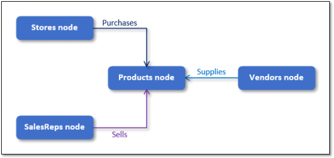
The data model includes only four nodes (Stores, SalesReps, Vendors, and Products) and only three edges (Purchases, Sells, and Supplies). Together these nodes and edges define the following relationships:
- Stores purchase products
- Sales reps sell products
- Vendors supply products
You’ll define these relationships within the edge tables by mapping the originating node to the terminating node for each relationship, as you saw in the first article in this series. The implication here is that you should first populate the node tables before the edge tables so you can reference the originating and terminating node IDs when defining your relationships.
Creating and Populating the Node Tables
Before you can create and populate your node tables, you must determine where to put the tables. For the examples in this article, I created the graph schema within the AdventureWorks2017 database, using the following T-SQL code:
|
1 2 3 4 |
USE AdventureWorks2017; GO CREATE SCHEMA graph; GO |
You do not need to locate the graph tables in the graph schema or even in the AdventureWorks2017 database. However, if you plan to try out the examples to follow and want to locate the graph tables elsewhere, be sure to update the T-SQL code accordingly.
With the graph schema in place (or wherever you locate the tables), you can then create and populate the Stores node table, which includes two user-defined columns, StoreID and StoreName, as shown in the following CREATE TABLE statement:
|
1 2 3 4 5 6 7 8 9 10 |
DROP TABLE IF EXISTS graph.Stores; GO CREATE TABLE graph.Stores ( StoreID INT PRIMARY KEY, StoreName NVARCHAR(50) NOT NULL ) AS NODE; INSERT INTO graph.Stores(StoreID, StoreName) SELECT c.CustomerID, s.Name FROM Sales.Customer c INNER JOIN Sales.Store s ON c.StoreID = s.BusinessEntityID; |
The example follows the same procedures used in the first article to create and populate node tables, so be sure to refer back to the article if you’re unsure about what we’re doing here. Keep in mind that you must include the AS NODE clause in the CREATE TABLE statement. You can also add whatever other user-defined columns you want to include. SQL Server will automatically generate the table’s $node_id column.
You can then use an INSERT…SELECT statement to populate the Stores table, as you would with any SQL Server table. In this case, you must join the Sales.Customer table to the Sales.Store table to get the store name. In addition, when supplying values for the StoreID column in the Stores table, you should use the CustomerID value in the Customer table, rather than use the StoreID value in that table, because the SalesOrderHeader table uses the CustomerID value. This approach helps to keep things simpler when populating the edge tables. SQL Server automatically populates the $node_id column.
That’s all there is to setting up the Stores table, and creating and populating the SalesReps table is even easier:
|
1 2 3 4 5 6 7 8 9 10 11 |
DROP TABLE IF EXISTS graph.SalesReps; GO CREATE TABLE graph.SalesReps ( SalesRepID INT PRIMARY KEY, FirstName NVARCHAR(50) NOT NULL, LastName NVARCHAR(50) NOT NULL, ) AS NODE; INSERT INTO graph.SalesReps(SalesRepID, FirstName, LastName) SELECT BusinessEntityID, FirstName, LastName FROM Person.Person WHERE PersonType = 'SP'; |
For this example, you can pull all the data directly from the Person table, limiting the results to those rows with a PersonType value of SP (for salesperson). If you want to include such information as sales quotas or job titles in the table, you must join the Person table to the SalesPerson or Employee table (or both). For this example, however, the Person table is enough.
The next table to create and populate is Products. For this, you can pull all the data from the Production.Product table:
|
1 2 3 4 5 6 7 8 9 10 11 |
DROP TABLE IF EXISTS graph.Products; GO CREATE TABLE graph.Products ( ProductID INT PRIMARY KEY, ProductName NVARCHAR(50) NOT NULL, StandardCost MONEY NOT NULL, ) AS NODE; INSERT INTO graph.Products(ProductID, ProductName, StandardCost) SELECT ProductID, Name, StandardCost FROM Production.Product WHERE FinishedGoodsFlag = 1; |
For this example, when retrieving data from the Product table, you should include a WHERE clause that filters the data so that only rows with a FinishedGoodsFlag value of 1 are included. This ensures that you include only salable products in the Products table.
The final node table is Vendors, which gets all its data from the Purchasing.Vendor table:
|
1 2 3 4 5 6 7 8 9 10 |
DROP TABLE IF EXISTS graph.Vendors; GO CREATE TABLE graph.Vendors ( VendorID INT PRIMARY KEY, AccountNumber NVARCHAR(15) NOT NULL, VendorName NVARCHAR(50) NOT NULL ) AS NODE; INSERT INTO graph.Vendors(VendorID, AccountNumber, VendorName) SELECT BusinessEntityID, AccountNumber, Name FROM Purchasing.Vendor; |
That’s all there is to creating and populating the node tables. Once they’re in place, you can start in on your edge tables.
Creating and Populating the Edge Tables
Creating an edge table is just as simple as a node table, with a few notable differences. For the edge table, the table definition requires an AS EDGE clause, rather than an AS NODE clause, and the user-defined columns are optional. (Node tables require at least one user-defined column.) In addition, SQL Server automatically generates the $edge_id column, rather than the $node_id column.
The first edge table is Orders, which includes three user-defined columns, as shown in the following CREATE TABLE statement:
|
1 2 3 4 5 6 7 |
DROP TABLE IF EXISTS graph.Orders; GO CREATE TABLE graph.Orders ( OrderDate DATETIME NOT NULL, OrderQty SMALLINT NOT NULL, LineTotal MONEY NOT NULL ) AS EDGE; |
After you create the Orders table, you can add the data, which relies on the SalesOrderHeader and SalesOrderDetail tables to supply the values for the user-defined columns and, more importantly, to provide the structure for defining the relationships between the Stores and Products nodes:
|
1 2 3 4 5 6 7 8 9 10 |
INSERT INTO graph.Orders($from_id, $to_id, OrderDate, OrderQty, LineTotal) SELECT s.node1, p.node2, h.OrderDate, d.OrderQty, d.LineTotal FROM Sales.SalesOrderHeader h INNER JOIN Sales.SalesOrderDetail d ON h.SalesOrderID = d.SalesOrderID INNER JOIN (SELECT $node_id AS node1, StoreID FROM graph.Stores) s ON h.CustomerID = s.StoreID INNER JOIN (SELECT $node_id AS node2, ProductID FROM graph.Products) p ON d.ProductID = p.ProductID; |
After joining the SalesOrderHeader and SalesOrderDetail tables, the SELECT statement joins the SalesOrderHeader table to the Stores tables, based on the CustomerID and StoreID values. The join uses a subquery to retrieve only the $node_id and StoreID columns from the Stores table and to rename the $node_id column to node1. The query will fail if you try to use $node_id in the SELECT list. You can then join the SalesOrderHeader table to the Products table, using the same logic as when joining to the Stores table.
The node1 and node2 columns returned by the SELECT statement provide the values for the $from_id and $to_id columns in the edge table. As you’ll recall from the first article, you must specifically provide these values when inserting data into an edge table. The values are essential to defining the relationships between the originating and terminating nodes. SQL Server automatically populates the $edge_id column.
The next step is to create and populate the Sells edge table, which works much the same way as the Orders table, even when it comes to the user-defined columns. The main difference is that the relationships originate with the SalesReps table, as shown in the following T-SQL code:
|
1 2 3 4 5 6 7 8 9 10 11 12 13 14 15 16 17 18 |
DROP TABLE IF EXISTS graph.Sells; GO CREATE TABLE graph.Sells ( OrderDate DATETIME NOT NULL, OrderQty SMALLINT NOT NULL, LineTotal MONEY NOT NULL ) AS EDGE; INSERT INTO graph.Sells($from_id, $to_id, OrderDate, OrderQty, LineTotal) SELECT s.node1, p.node2, h.OrderDate, d.OrderQty, d.LineTotal FROM Sales.SalesOrderHeader h INNER JOIN Sales.SalesOrderDetail d ON h.SalesOrderID = d.SalesOrderID INNER JOIN (SELECT $node_id AS node1, SalesRepID FROM graph.SalesReps) s ON h.SalesPersonID = s.SalesRepID INNER JOIN (SELECT $node_id AS node2, ProductID FROM graph.Products) p ON d.ProductID = p.ProductID; |
The fact that the Orders and Sells tables include the same user-defined columns points to the possibility that you could create a fifth node table for sales orders and then include columns such as OrderDate in there. However, this approach could make your schema and queries unnecessarily complicated, while providing little benefit. On the other hand, this approach helps to eliminate duplicate data. As with any database, the exact layout of your graph model will depend on the type of data you’re storing and how you plan to query that data.
The last step is to create and populate the Supplies table. In this case, the structure for the relationships is available through the ProductVendor table:
|
1 2 3 4 5 6 7 8 9 10 11 12 13 14 |
DROP TABLE IF EXISTS graph.Supplies; GO CREATE TABLE graph.Supplies ( StandardPrice MONEY NOT NULL ) AS EDGE; INSERT INTO graph.Supplies($from_id, $to_id, StandardPrice) SELECT v.node1, p.node2, pv.StandardPrice FROM Purchasing.ProductVendor pv INNER JOIN (SELECT $node_id AS node1, VendorID FROM graph.Vendors) v ON pv.BusinessEntityID = v.VendorID INNER JOIN (SELECT $node_id AS node2, ProductID FROM graph.Products) p ON pv.ProductID = p.ProductID; |
The ProductVendor table does all the product-vendor mapping for you and includes the StandardPrice values. You need only join this table to the Vendors and Products tables to get the originating and terminating node IDs.
Retrieving Store Sales Data
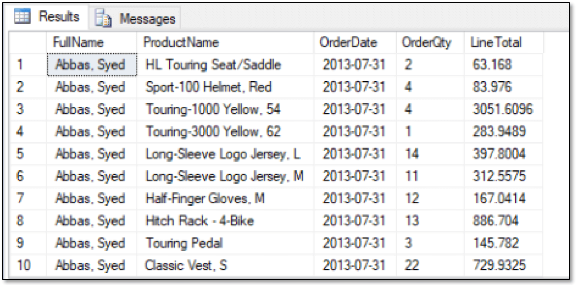
With the graph tables now defined and populated, you’re ready to start querying them, just like you saw in the second article in this series. For example, you can use the following SELECT statement to return information about the products that each store has ordered:
|
1 2 3 4 5 |
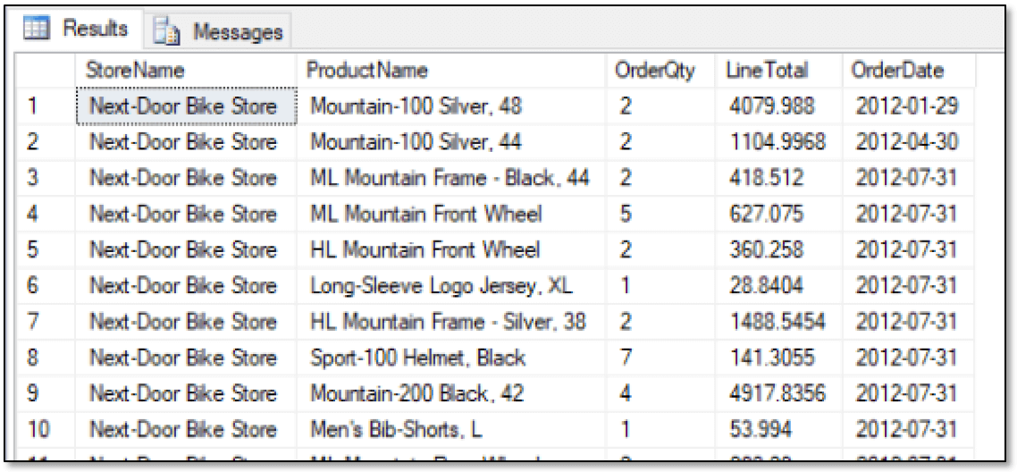
SELECT s.StoreName, p.ProductName, o.OrderQty, o.LineTotal, CAST(o.OrderDate AS DATE) AS OrderDate FROM graph.Stores s, graph.Orders o, graph.Products p WHERE MATCH(s-(o)->p) ORDER BY s.StoreID; |
The SELECT statement uses the MATCH function to specify what data to retrieve. As described in the second article, the function lets you define a search pattern based on the relationships between nodes. You can use the function only in the WHERE clause of a query that targets node and edge tables. The following table shows part of the results that the SELECT statement returns. (The statement returns over 60,000 rows.)
In the above example, the MATCH clause specifies the relationship store orders product. If you were to retrieve the same data directly from the relational tables, you could not use the MATCH clause. Instead, your query would look similar to the following:
|
1 2 3 4 5 6 7 8 9 |
SELECT c.CustomerID, c.StoreID, st.Name StoreName, p.name ProductName, d.OrderQty, d.LineTotal, s.OrderDate FROM sales.SalesOrderHeader s INNER JOIN sales.SalesOrderDetail d ON s.SalesOrderID = d.SalesOrderID INNER JOIN sales.customer c ON s.CustomerID = c.CustomerID INNER JOIN sales.store st ON c.storeid = st.BusinessEntityID INNER JOIN production.product p ON d.ProductID = p.ProductID WHERE p.FinishedGoodsFlag = 1 ORDER BY st.BusinessEntityID; |
Although this query is more complex than the previous one, you can use it without having to create and populate graph tables. As with any data, you’ll have to determine on a case-by-case basis when a graph database will be useful to your circumstances and which structure will deliver the best-performing queries.
Returning now to the graph tables, you can modify the preceding example by grouping the data based on the stores and products, as shown in the following example:
|
1 2 3 4 5 6 7 |
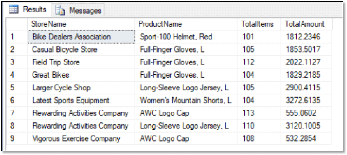
SELECT s.StoreName, p.ProductName, SUM(o.OrderQty) AS TotalItems, SUM(o.LineTotal) AS TotalAmount FROM graph.Stores s, graph.Orders o, graph.Products p WHERE MATCH(s-(o)->p) GROUP BY s.StoreName, p.ProductName HAVING SUM(o.OrderQty) > 100 ORDER BY s.StoreName; |
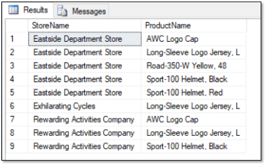
As you can see, you can use the MATCH function in conjunction with other clauses, including the HAVING clause, which in this case, limits the results to rows with a total quantity greater than 100. The following figure shows the data now returned by the SELECT statement.
When implementing a graph database based on existing relational data, you might want to copy only part of the data set into the graph tables, in which case, you’ll likely need to create queries that can retrieve data from both the graph and relational tables. One way to achieve this is to define a common table expression (CTE) that retrieves the graph data and then use the CTE when retrieving the relational data, as shown in the following example:
|
1 2 3 4 5 6 7 8 9 10 11 12 13 14 15 16 17 18 |
WITH StoreOrders AS ( SELECT s.StoreName, p. ProductID, p.ProductName, SUM(o.OrderQty) AS TotalItems, SUM(o.LineTotal) AS TotalAmount FROM graph.Stores s, graph.Orders o, graph.Products p WHERE MATCH(s-(o)->p) GROUP BY s.StoreName, p.ProductID, p.ProductName HAVING SUM(o.OrderQty) > 100 ) SELECT so.StoreName, so.ProductName, ps.Name AS ProductSubcategory, pc.Name AS ProductCategory, so.TotalItems, so.TotalAmount FROM StoreOrders so INNER JOIN Production.Product pr ON so.ProductID = pr.ProductID INNER JOIN Production.ProductSubcategory ps ON pr.ProductSubcategoryID = ps.ProductSubcategoryID INNER JOIN Production.ProductCategory pc ON ps.ProductCategoryID = pc.ProductCategoryID ORDER BY so.StoreName; |
In this case, the outer SELECT statement joins the data from the CTE to the Product, ProductSubcategory, and ProductCategory tables in order to include the product categories and subcategories in the results, as shown in the following figure.
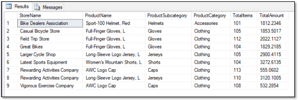
Being able to access both graph and relational data makes it possible to implement a graph database for those complex relationships that can justify the additional work, while still retaining the basic relational structure for all other data.
Retrieving Sales Rep and Vendor Data
Of course, once you have your graph tables in place, you can run a query against any of them. For example, the following query returns a list of sales reps and the products they have sold, along with details about the orders:
|
1 2 3 4 5 |
SELECT r.LastName + ', ' + r.FirstName AS FullName, p.ProductName, CAST(s.OrderDate AS DATE) AS OrderDate, s.OrderQty, s.LineTotal FROM graph.SalesReps r, graph.Sells s, graph.Products p WHERE MATCH(r-(s)->p) ORDER BY r.LastName, r.FirstName; |
As you can see, retrieving information about the Sells relationships works just like returning data about the Orders relationships, but now the results are specific to each sales rep, as shown in the following figure.
The results shown here are only a small portion of the returned data. The statement actually returns over 60,000 rows. However, you can aggregate the data just as you saw earlier:
|
1 2 3 4 5 6 7 8 |
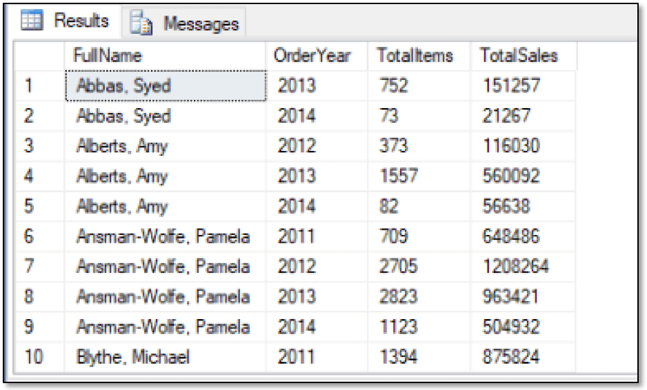
SELECT r.LastName + ', ' + r.FirstName AS FullName, YEAR(s.OrderDate) AS OrderYear, SUM(s.OrderQty) AS TotalItems, CAST(SUM(s.LineTotal) AS INT) AS TotalSales FROM graph.SalesReps r, graph.Sells s, graph.Products p WHERE MATCH(r-(s)->p) GROUP BY r.LastName, r.FirstName, YEAR(s.OrderDate) ORDER BY r.LastName, r.FirstName, YEAR(s.OrderDate); |
Now the SELECT statement returns only 58 rows, with the first 10 shown below.
There’s little difference between returning data based on the Orders relationships or the Sells relationships, except that the originating nodes are different. You can also take the same approach to retrieve vendor data. Just be sure to update the table alias references as necessary, as shown in the following example:
|
1 2 3 4 5 6 7 8 9 10 11 12 13 14 15 16 17 18 |
WITH VendorProducts AS ( SELECT v.VendorName, p.ProductID, p.ProductName, AVG(s.StandardPrice) AvgPrice FROM graph.Vendors v, graph.Supplies s, graph.Products p WHERE MATCH(v-(s)->p) GROUP BY v.VendorName, p.ProductID, p.ProductName ) SELECT vp.VendorName, vp.ProductName, ps.Name AS ProductSubcategory, pc.Name AS ProductCategory FROM VendorProducts vp INNER JOIN Production.Product pr ON vp.ProductID = pr.ProductID INNER JOIN Production.ProductSubcategory ps ON pr.ProductSubcategoryID = ps.ProductSubcategoryID INNER JOIN Production.ProductCategory pc ON ps.ProductCategoryID = pc.ProductCategoryID WHERE pc.Name = 'Components' ORDER BY vp.VendorName, vp.ProductName; |
This should all look familiar to you. The SELECT statement uses a CTE to join the graph and relational data together. The following table shows the first 10 rows of the 32 that the statement returns.
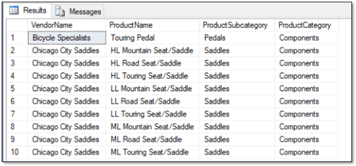
As you can see, the results include the vendor and product names, along with the product subcategories and categories.
Digging into the Graph Data
Once you get the basics down of how to query your graph tables, you can come up with other ways to understand the relationships between the nodes. For example, the following SELECT statement attempts to identity sales reps who might be focusing too heavily on certain vendors:
|
1 2 3 4 5 6 7 8 9 |
SELECT r.LastName + ', ' + r.FirstName AS FullName, v.VendorName, CAST(SUM(sl.LineTotal) AS INT) AS TotalAmount FROM graph.SalesReps r, graph.Sells sl, graph.Products p, graph.Supplies sp, graph.Vendors v WHERE MATCH(r-(sl)->p<-(sp)-v) GROUP BY r.LastName, r.FirstName, v.VendorName HAVING SUM(sl.LineTotal) > (SELECT AVG(LineTotal) FROM graph.Sells) * 50 ORDER BY r.LastName, r.FirstName, v.VendorName; |
The statement groups the data by the name of the sales reps and then by the vendors. The statement also includes a HAVING clause that calculates an amount 50 times the average sales and then compares that to the total sales of each sales rep. Only reps that go over the calculated amount are included in the results, as shown in the following figure.
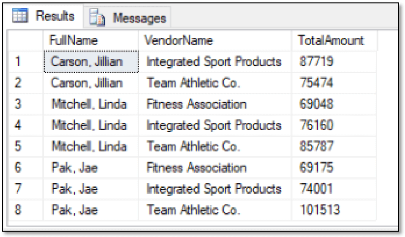
By being able to return this type of information, you can identify patterns that point to anomalies or specific trends in the data set. For instance, suppose you now want to identify the products that stores have bought based on a specified product that they also bought (a scenario sometimes referred to customers who bought this also bought that).
One way to get this information is to use a CTE to retrieve the IDs of the stores that ordered the specified product and then, for each store return the list of other products that the store ordered. To achieve this, use the CTE to qualify your query so it returns only the other products that the stores bought:
|
1 2 3 4 5 6 7 8 9 10 11 12 13 14 15 16 17 |
WITH StoreIDs AS ( SELECT s.StoreID FROM graph.stores s, graph.Orders o, graph.Products p WHERE MATCH(s-(o)->p) AND p.ProductName = 'Sport-100 Helmet, Blue' GROUP BY s.StoreID, s.StoreName HAVING SUM(o.OrderQty) > 75 ) SELECT s.StoreName, p.ProductName FROM graph.stores s, graph.Orders o, graph.Products p WHERE MATCH(s-(o)->p) AND s.StoreId IN (SELECT StoreID FROM StoreIDs) AND p.ProductName <> 'Sport-100 Helmet, Blue' GROUP BY s.StoreName, p.ProductName HAVING SUM(o.OrderQty) > 75 ORDER BY StoreName, ProductName; |
The outer SELECT statement returns the list of products that each of the three stores has ordered. The key is to use the IN operator in a WHERE clause condition to compare the StoreId value to a list of store IDs returned by the CTE. You should also include a WHERE clause condition to exclude the product Sport-100 Helmet, Blue. The SELECT statement returns the results shown in the following figure.
There are other ways you can get at customers who bought this also bought that information, such as using Python or R, but this approach provides a relatively simple way to get the data from a graph database, without having to jump through too many hoops.
Making the Best of Both Worlds
Because the graph database features are integrated with the database engine, there’s no reason you can’t work with graph and relational data side-by-side, depending on your application requirements and the nature of your data. This integration also gives you the flexibility to incorporate graph tables into an existing relational structure or make them both part of the design when planning for a new application. Keep in mind, however, that the graph features are still new to SQL Server and lack some of the advanced capabilities available to more established graph products. Perhaps after a couple more releases, SQL Server will be a more a viable contender in the graph database market, at least when used in conjunction with relational data.
FAQs: SQL Server Graph Databases – Part 5: Importing Relational Data into a Graph Database
1. How do I import relational data into a SQL Server graph database?
Create node tables (AS NODE) for each entity type in your relational model, then create edge tables (AS EDGE) for each relationship. Populate the node tables using INSERT…SELECT from your existing relational tables. For edge tables, join the source and target node tables to get the internal $node_id values for each relationship, then insert those pairs into the edge table. You can query the graph tables immediately using the MATCH clause.
2. What is the MATCH clause in SQL Server graph queries?
The MATCH clause is used in SELECT statements to specify relationship patterns between graph node and edge tables. It uses an arrow notation – MATCH(NodeA-(Edge)->NodeB) – to express that NodeA has an edge relationship pointing to NodeB. You can chain multiple MATCH conditions to traverse multiple relationship hops in a single query, which would otherwise require multiple JOINs in a relational model.
3. Can I use graph tables and relational tables in the same SQL Server query?
Yes. SQL Server graph tables are stored in the same database as regular relational tables and can be JOINed together in standard SELECT statements. You can use MATCH to navigate the graph portion of a query while JOINing to regular relational tables for additional data. This allows incremental adoption – you can add graph relationships to an existing relational database without migrating all data to a pure graph structure.
4. What SQL Server version do I need for graph database features?
Graph database features (AS NODE, AS EDGE, and MATCH) were introduced in SQL Server 2017. The SHORTEST_PATH function and other advanced graph features were added in SQL Server 2019. For most import and query scenarios, SQL Server 2017 is the minimum requirement. Azure SQL Database and SQL Managed Instance also support SQL Server graph features.
This document contains proprietary information and is protected by copyright law.
Copyright © 2026 Red Gate Software Limited. All rights reserved


Load comments