In the modern data landscape, most of the effort doesn’t go into building models or dashboards. It goes into getting the data into a usable state. Generally, a large portion of time is spent extracting, cleaning, and reshaping data before any analysis can begin. While Python and SQL together form a powerful stack, the boundary between them is often where things start to break down.

In this article, you’ll learn how to build a more reliable flow by pushing the right work into SQL and keeping Python focused on what it does best: analysis. Plus, expert tips and advice on views, CTEs, pruning, and efficient data extraction.

The foundation: establishing the ‘contract’ layer

A robust pipeline requires an abstraction layer that shields downstream scripts from underlying database fragility.

Views as analytical contracts

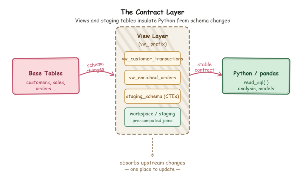
One of the most underused patterns in data engineering is database views, specifically as a stable contract between SQL schema and Python. When we write queries directly against base tables, the Python scripts inherit every structural assumption baked into those tables. A renamed column, a modified join, or a schema migration can silently break downstream logic.

The practical fix involves introducing a dedicated view layer – typically prefixed with vw_ – that the Python code can query instead. These views absorb upstream schema changes. By updating the view definition in just one place, everything downstream can continue to function without modification when an underlying table evolves. Effectively, the view becomes the agreed-upon representation of the data rather than just a passthrough.

For Python’s script, the underlying tables don’t really exist. The script only interacts with vw_customer_transactions. Without this layer, analytical logic such as joins and filters tend to leak into Python and become redefined across multiple scripts.

The workspace schema explained

For multi-step or computation-heavy transformations, relying on on-the-fly joins inside extraction queries is inefficient and difficult to maintain. Instead, introduce a ‘workspace schema’ dedicated to intermediate analytical work. This way, pre-computations are isolated into a controlled namespace rather than cluttering the primary schema with temporary logic. This makes it immediately clear which objects are ephemeral and keeps the catalog clean.

In SQL Server, this can be implemented using schema-qualified staging tables (or GlobalTempTables) for cross-session visibility. The idea is simple: compute expensive joins once, then reuse the result.

Consider a churn prediction dataset where relevant features span multiple tables. Recomputing joins every time a feature changes is wasteful. Instead:

During iterative development, this approach avoids repeatedly paying the cost of complex joins. You compute just once per session, so subsequent extractions become lightweight and fast.

Explaining logical abstraction with common table expressions (CTEs)

As SQL queries grow, deeply nested logic quickly becomes unreadable and fragile. Common Table Expressions (CTEs) provide a way to modularize SQL logic, much like functions do in application code. Using the WITH clause, we define named intermediate steps that isolate distinct parts of the transformation.

Instead of a monolithic query, build a sequence of logical steps that are easier to read, debug and modify. CTEs act as a structural guide through complex transformations, ensuring that by the time data reaches Python, its lineage and logic are already clear.

The gatekeeper: source-side data integrity

The database should act as a strict bouncer. This is to ensure that only pristine, necessary data is allowed into the memory buffer.

Dimensional pruning explained

The first rule of data extraction is simple: don’t pull what you don’t need. Yet, in practice, SELECT * still shows up in production pipelines far too often.

Vertical pruning (projection pushdown) means only selecting the columns your downstream logic actually requires. If a table has 40 columns and you use 8, for example, the remaining 32 columns represent unnecessary network transfer, deserialization, and memory usage.

Horizontal pruning (predicate pushdown) means applying filters as early as possible using WHERE clauses. When filtering happens in SQL, the database engine can leverage indexes and eliminate rows before they’re transmitted. When filtering happens in Python, the cost has already been incurred.

String sanitization explained

Text data is often inconsistent and can create significant downstream issues. Cleaning strings at the database level avoids unnecessary work in Python and ensures consistency across all consumers.

For example: TRIM(LOWER(email)) standardizes casing and removes whitespace before the data ever leaves the database. The equivalent in Pandas, df['email'].str.strip().str.lower(), does work, but only after the data has already been transferred and loaded into memory.

More importantly, normalization at the source ensures correctness. If two records differ only by casing (e.g User@Example.com vs user@example.com), they will not join correctly unless standardized. Handling this in SQL guarantees consistency regardless of which script consumes the data.

Strict type enforcement

Python’s performance model depends on consistent, predictable data types, especially when working with Pandas or NumPy. Weak or implicit typing at the SQL layer often leads to subtle downstream issues that are difficult to debug.

An example is SQL Server’s BIT type being interpreted inconsistently in Python, sometimes appearing as integers (0/1) instead of boolean values. Similarly, numeric fields may be inferred as object types if NULL values are present, which breaks vectorized operations and slows computation.

The fix is to enforce type consistency at the source. Using explicit casting ensures that the data arrives in Python exactly as expected:

Equally important is handling missing values proactively. Leaving NULL values unmanaged often results in unintended NaN propagation in Pandas, which can silently alter aggregations or model inputs.

Once data enters Python, type inconsistencies become exponentially harder to trace because they manifest during transformations rather than at ingestion.

The engine: leveraging set-based logic to eliminate heavy Python compute

Relational databases are highly optimized for set-based logic. Offloading the compute to the database engine saves massive amounts of CPU overhead in Python.

Temporal alignment with window functions

Time-series analysis in Python often involves operations like computing the previous value, calculating rolling averages, or ranking records within groups. The typical approach is to extract raw data and apply Pandas shift(), rolling(), or groupby().rank(). Window functions allow you to push this entire class of computation into the database engine, where it can be executed more efficiently as part of a set-based query.

Consider a scenario where a team needs to analyze a sudden 20% drop in pre-orders for a product. A naive approach would involve pulling daily sales into Python and computing week-over-week changes. The better solution is to compute this directly in SQL:

Here, the database aggregates, aligns temporal context and computes comparative metrics all before the data ever reaches Python. The result is a time-series dataset usable for analysis or modeling.

Statistical pre-processing explained

Databases natively support statistical functions like standard deviation, variance and percentile ranks, etc. When the goal is to prepare data for modeling rather than explore it interactively, computing these metrics in SQL is often more efficient.

This also applies to A/B testing workflows. Rather than extracting raw event-level data, you can compute per-group aggregates, counts, means and variances directly in SQL. Then, you can send a compact summary to Python for hypothesis testing. The result is less data movement and a clearer separation of responsibilities between systems.

Complex data flattening explained

Modern schemas often include semi-structured data such as JSON, arrays, or nested attributes. Parsing these structures in Python introduces unnecessary overhead and typically results in row-by-row processing, which is slow and difficult to maintain. SQL, on the other hand, provides native operators for working with these types.

This produces a flat, tabular dataset without navigating nested structures in Python.

The extraction: performance and throughput

When the data is clean and flattened, the physical transfer method dictates the speed of pipeline.

Vectorized transfers explained

Traditional row-by-row cursors like standard psycopg2 (or similar adaptors) introduce significant overhead, because each row is deserialized individually. Modern data pipelines favor columnar, vectorized transfers, often using Apache Arrow as the underlying format.

Libraries like Polars, combined with high-performance connectors such as ConnectorX, allow data to be loaded directly into memory in a columnar layout. This significantly improves throughput and reduces CPU overhead for enterprise scale. In practice, this can reduce extraction times dramatically without changing the SQL query itself.

Extraction strategy selection

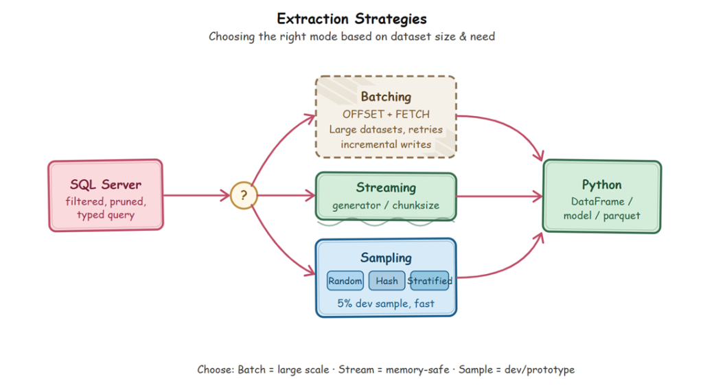
The optimal extraction strategy in databases depends on data size and processing requirements. Batching, for example, splits large datasets into manageable chunks using OFFSET and FETCH. This means repeatedly querying ordered slices of data (e.g., ORDER BY order_id LIMIT n OFFSET k), which supports incremental writes, retrying failed batches, and progress tracking. However, large offsets can degrade performance.

An alternative is Streaming, which avoids this issue by consuming results incrementally using Python generators and chunked reads (chunksize) from a single query. It yields values one at a time rather than returning everything at once. Memory usage remains stable because only one chunk is processed at a time. This is the preferred approach when processing is sequential and doesn’t require random access.

Stratification and sampling

When prototyping machine learning models or testing pipeline logic, analyzing the entire ‘Big Data’ warehouse is counterproductive and wastes expensive compute resources. A smaller, representative subset is enough – plus, it’s significantly faster to iterate on. There are three distinct sampling strategies, each serving a different purpose:

Random sampling is the simplest approach. Most databases support this directly through constructs like TABLESAMPLE (n PERCENT), which returns an approximate fraction of rows. It’s fast and easy to use, but not reproducible.

For reproducibility matters such as debugging or consistent experimentation, deterministic sampling is more reliable. This is typically done by hashing a stable identifier (e.g., HASHTEXT(customer_id)). Because the hash output is consistent, the same subset of records is selected every time.

Stratified sampling is used when the dataset is imbalanced. Instead of sampling globally, the data is partitioned into groups (e.g., PARTITION BY is_fraud) and sampling is applied within each group. This is commonly implemented using window functions like ROW_NUMBER() to select a proportional subset from each category. This ensures that both majority and minority classes are preserved in the final sample.

Consider fraud detection, where fraudulent transactions might represent only 0.3% of total data. A naive random sample may include too few fraud cases to be useful. Stratified sampling ensures that each subgroup is proportionally represented.

Putting it all together

Across all these patterns, the principle remains consistent. SQL databases are optimized for transformation, filtering, and aggregation. Python is optimized for modeling, statistical analysis, and application logic.

The extraction layer is where responsibility shifts from one system to the other. When this boundary is designed deliberately using contracts, pruning, pre-computation, and efficient transfer mechanisms, you spend less time maintaining pipelines and more time doing meaningful analysis.

None of these ideas are individually complex. The difference comes from applying them intentionally, rather than defaulting into patterns that seem convenient in the moment but fail under scale.

References

- Shan, J., Goldwasser, M., Malik, U., & Johnston, B. (2022). SQL for data analytics (3rd ed.)
- Illinghton, A. (2024). Python programming and SQL: 6 books in 1
Simple Talk is brought to you by Redgate Software
FAQs: How to get clean, usable data out of SQL Server into Python
1. Why should data transformations be pushed into SQL instead of Python?
SQL engines are optimized for set-based operations like filtering, joining, and aggregation. Performing these tasks in SQL reduces data transfer, improves performance, and simplifies Python code.
2. What is a “contract layer” in data pipelines?
A contract layer (often implemented with database views) acts as a stable interface between raw tables and downstream code, protecting pipelines from schema changes.:
3. How do database views improve pipeline reliability?
Views abstract underlying schema complexity. When base tables change, only the view needs updating—downstream Python scripts remain unaffected.
4. What is dimensional pruning and why does it matter?
Dimensional pruning means selecting only required columns (vertical) and rows (horizontal). This reduces memory usage, speeds up queries, and minimizes unnecessary data transfer.
5. Why should data cleaning (e.g., string normalization) happen in SQL?
Cleaning data at the source ensures consistency across all consumers and avoids redundant processing in Python after data is loaded.
6. What are Common Table Expressions (CTEs) used for?
CTEs modularize complex SQL queries into readable steps, making transformations easier to debug, maintain, and extend.
7. When should you use a workspace or staging schema?
Use it for heavy joins or intermediate computations that are reused multiple times, improving performance and keeping production schemas clean.
8. How do window functions improve performance?
Window functions handle time-based calculations (like rolling averages or lag comparisons) directly in SQL, eliminating the need for expensive Python computations.
9. What is the best way to extract large datasets efficiently?
Use vectorized, columnar transfers (e.g., Apache Arrow-based tools) or streaming approaches instead of row-by-row extraction to improve speed and reduce memory usage.
10. What sampling strategies are best for large datasets?
- Random sampling for quick exploration
- Deterministic sampling for reproducibility
- Stratified sampling for imbalanced datasets (e.g., fraud detection)
This document contains proprietary information and is protected by copyright law.
Copyright © 2026 Red Gate Software Limited. All rights reserved
Load comments