When Microsoft Fabric was born, the only method to convert files to tables was using notebooks. Nowadays we have an easy-to-use UI feature for the conversion.

As I explained on the article about lakehouse and ETL, there are some scenarios where we still need to use notebooks for the conversion. One of these scenarios is when we need table partitioning.

Let’s make a step-by-step on this blog about how to use notebooks and table partitioning.

The steps explained here are based on the same sample data from the lakehouse and ETL article. In that article you can find the steps to build a pipeline to import the data to the files area.

The Starting Point

The starting point for this example is a lakehouse called demolake with the files already imported to the Files area using a pipeline.

No table is created yet.

Loading a Notebook

We will use a notebook for the conversion. You can download the notebook here. We will use the notebook called “01 – Create Delta Tables.ipynb”

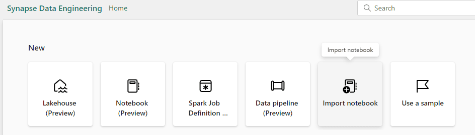
1. Click the Experience button and select the Data Engineering Experience
2. Click the Import Notebook button.

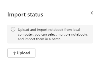
1. Click the Upload button and select the notebook you just downloaded.

1. Click the button lakehouse demo in the left button bar to return to the workspace.

1. Click on the notebook you imported.
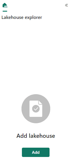
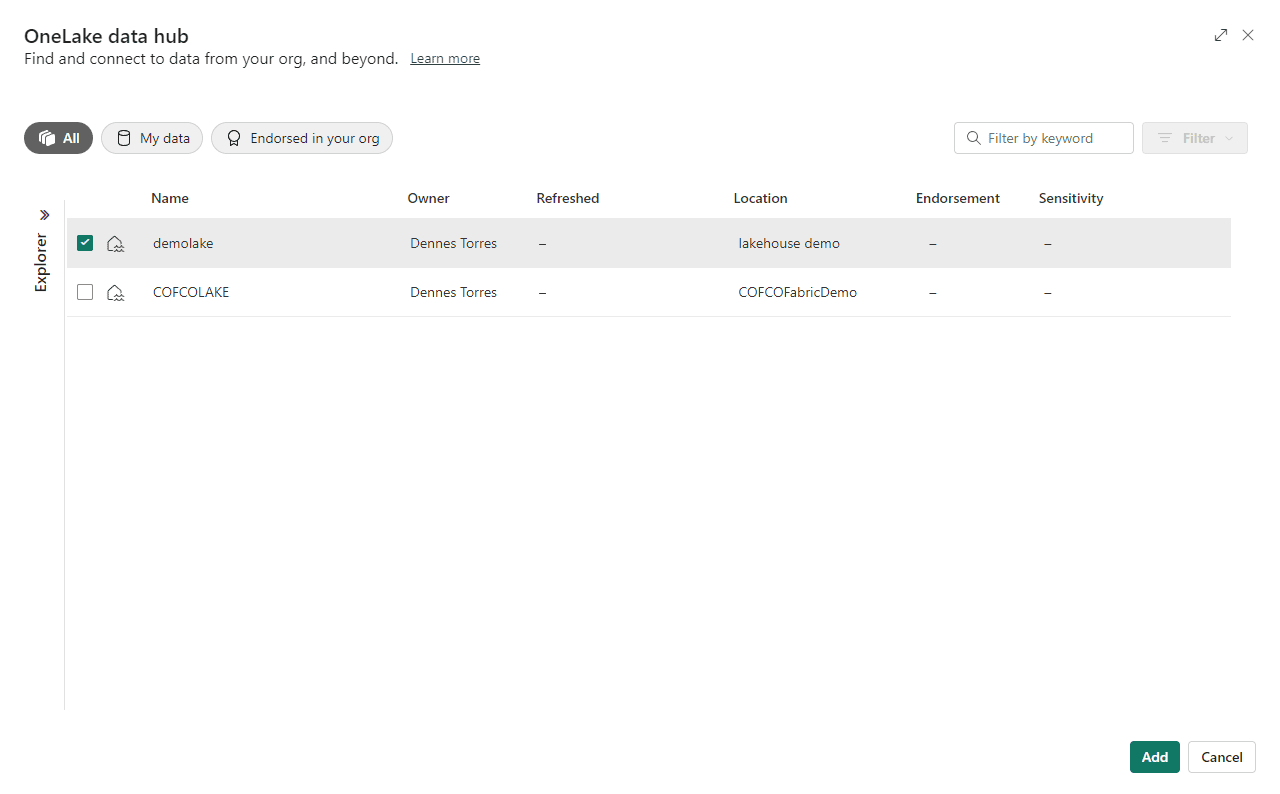
2. On the Lakehouse explorer window, click the Add button to link the notebook to a lakehouse.

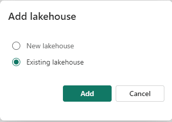
1. On the Add Lakehouse window, select Existing Lakehouse and click the Add button.

1. Select the demolake and click the Add button.

The notebook code

Let’s analyse the code in the notebook we just imported.

First Code Block

# Copyright (c) Microsoft Corporation.
# Licensed under the MIT License.

spark.conf.set("sprk.sql.parquet.vorder.enabled", "true")

spark.conf.set("spark.microsoft.delta.optimizeWrite.enabled", "true")

spark.conf.set("spark.microsoft.delta.optimizeWrite.binSize", "1073741824")

This code block enables the V-Order optimization. This is a special optimization for delta tables. You can read more about the V-Order optimization on this link: https://learn.microsoft.com/en-us/fabric/data-engineering/delta-optimization-and-v-order?tabs=sparksql

The optimizeWrite option allow us to define what’s called binSize. This configuration defines the size for each parquet file used to store the data. Controlling the size of the files we can avoid too big files or too small files, either of these cases would cause a performance problem.

I would not be surprised if in the future some of these configurations may become a default.

Second Code Block

from pyspark.sql.functions import col, year, month, quarter

table_name = 'fact_sale'

df = spark.read.format("parquet").load('Files/fact_sale_1y_full')

df = df.withColumn('Year', year(col("InvoiceDateKey")))

df = df.withColumn('Quarter', quarter(col("InvoiceDateKey")))

df = df.withColumn('Month', month(col("InvoiceDateKey")))

df.write.mode("overwrite").format("delta").partitionBy("Year","Quarter").save("Tables/" + table_name)

This block executes the following tasks:

• Read the fact_sale table from the Files folder.
• Create a column called Year.
• Create a column called Quarter.
• Create a column called Month.
• Save the data in the Tables area. The table is partitioned by Year and Quarter, and it will overwrite any existing table with the same name.

Third Code Block

from pyspark.sql.types import *
def loadFullDataFromSource(table_name):
    df = spark.read.format("parquet").load('Files/' + table_name)
    df.write.mode("overwrite").format("delta").save("Tables/" + table_name)

full_tables = [

'dimension_city',
'dimension_date',
'dimension_employee',
'dimension_stock_item'
 ]

for table in full_tables:
    loadFullDataFromSource(table)

This block has a function called loadFullDataFromSource. The function is defined in the beginning of the code, but it will only be executed when called.

The execution itself starts on the full_tables variable definition. This variable is an array with the name of the dimensions, which are also the name of the folders under the Files area in the lakehouse.

A FOR loop is executed over the table variable. For each dimension, the function loadFullDataFromSource is called receiving the name of the dimension as a parameter.

The function loads the data from the Files area and saves it to the Tables area using the table name as parameter. As a result, the function will load all the dimensions, one by one.

Executing the Notebook and checking the result

1. Click the Run All button to execute all the code blocks in the notebook.

Microsoft Fabric uses a feature called Live Pool. We don’t need to configure a spark pool for the notebook execution. Every workspace linked with Fabric artifacts has the Live Pool enabled. Once we ask to execute a notebook or a single code block, the pool is enabled in very few seconds.

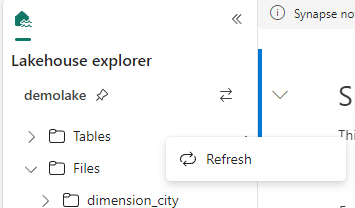
1. On the lakehouse explorer, right click Tables and click Refresh.

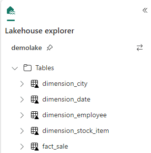
1. The tables are now available in the Tables area.

1. On the left bar, click the demolake button.

Let’s look on the storage behind the tables in the lakehouse.

1. Right click the fact_sale table
2. On the context menu, click View files menu item.

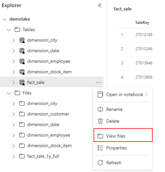
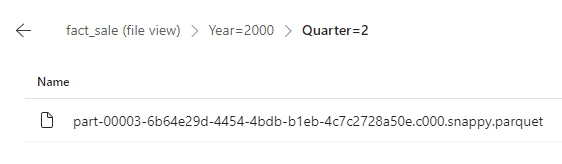
Mind how the files are stored in delta format and partitioned by Year and Quarter according to the configuration defined in the notebook.

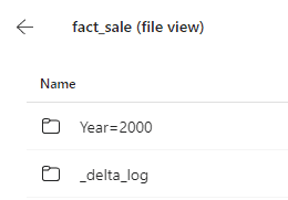
1. Click the Year folder.

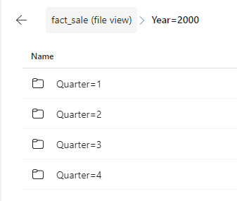
1. Click one of the Quarters folder.

Conclusion

On this blog you discovered how you can make the transformation from Files to Tables in a lakehouse using pyspark code and in this way be able to partition tables and schedule the code to make this movement.