SQL is a declarative language, designed to work with sets of data. However, it does support procedural, “row-by-row” constructs in the form of explicit cursors, loops and so on. The use of such constructs often offers the most intuitive route to the desired SQL solution, especially for those with backgrounds as application developers. Unfortunately, the performance of these solutions is often sub-optimal; sometimes very sub-optimal.

Some of the techniques used to achieve fast SQL code, and avoid row-by-row processing can, at first, seem somewhat obscure. This, in turn, raises questions over the maintainability of the code. However, in fact, there are really only a handful of these techniques that need to be dissected and understood in order to open a path towards fast, efficient SQL code. The intent of this article is to investigate a very common “running total” reporting problem, offer some fairly typical “procedural” SQL solutions, and then present much faster “set-based” solutions and dissect the techniques that they use.

The examples in this article are based on the classic “running total” problem, which formed the basis for Phil Factor’s first SQL Speed Phreak Competition. This challenge is not some far-fetched scenario that you will never encounter in reality, but a common reporting task, similar to a report that your boss may ask you to produce at any time.

In my experience, I’ve mostly found that the ease of producing the solution is inversely proportional to its performance and scalability. In other words, there is an easy solution and a fast solution, as well as many solutions in between. One may argue that for a report that runs once a month, clarity and maintainability are as important as speed, and there is some truth is this. However, bear in mind that while you can get away with a simple solution on a table with a few thousand rows, it won’t scale. As the number of rows grows so the performance will degrade, sometimes exponentially.

Furthermore, if you don’t know what’s possible in terms of performance, then you have no basis to judge the effectiveness of your solution. Once you’ve found the fastest solution possible then, if necessary, you can “back out” to a solution that is somewhat slower but more maintainable, in full knowledge of the size of the compromise you’ve made.

The Subscription List Challenge

The Subscription List challenge, as presented in Phil Factor’s Speed Phreak competition, consisted of one table containing a list of subscribers, with the dates that the subscribers joined, and the dates that they cancelled their subscription. The task was to produce a report, by month, listing:

• The number of new subscriptions
• The number of subscribers who have left
• A running total of current subscribers

Just about anything you wished to do was allowed in this challenge. You could use any version of SQL Server, change the indexes on the original table, use temp tables, or even use cursors. The person whose T-SQL solution returned the correct results in the fastest time was the winner.

In a nice twist, Phil Factor reported the standings daily and allowed multiple submissions. This allowed the entrants to fine-tune their solutions, and to help out some of the other contestants. The original solutions were developed against a sample dataset of 10,000 rows. However, the top entries performed so well that they were also tested against a 1 million row dataset. Likewise, all of the solutions in this were developed against the 10K-row dataset, but tested against both.

The eventual winner was Peso, the SQL Server MVP Peter Larsson, whose solution we will present and dissect, and which returned the required report, running against a 1 million row table, in just over 300 milliseconds. Eight other entrants ran very close, with solutions that ran in under 600 milliseconds.

Speed was all important in this contest; this was a super-charged drag race and there was little point turning up to the starting line in a mini-van. However, for lesser SQL mortals, you could be forgiven for regarding Peso’s winning solution with an equal mix of amazement and confusion. Hopefully, after reading the rest of this article, the solution will be clearer and the techniques accessible to you in solving your own T-SQL problems.

Setting Up

All you need to do to get started is to:

1. Create a new database in your test or development SQL Server instance.
2. Download the sample data from http://ask.sqlservercentral.com/questions/92/the-subscription-list-sql-problem.
3. Play the script found in the download to create and populate the table in your sample database.

Go ahead and take a look at the data by running SELECT * FROM Registrations. Figure 1 shows a sample of the data that we will be using to create the report.

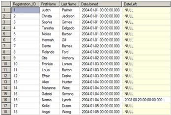
Figure 1: The data found in the Registrations table

Notice that many registrations do not have a DateLeft value. These subscriptions are ongoing and are active past the time period required for the report.

Validation

In order to prove that our solution works, we need to know what the correct answer should look like. In this case, of course, we could simply run Peso’s winning script. However, in practice, we won’t have that script and so we’ll need to do our own investigation of the data, to make sure we fully understand the report’s requirements.

The report must provide a list of the months, from the beginning of the data to the month of the contest (September, 2009), along with the count of new subscribers and cancellations for each month. After September 2009, there are no new registrations, only cancellations. The report must also supply a running total of the number of active subscriptions. The simple calculation for the number of active subscriptions in a given month is:

Number of subscriptions from previous month
+ new subscribers in current month
– cancellations in current month

To get started, run these two queries from Listing 1:

Listing 1: Another look at the data

Figure 2 shows the partial results. The first query shows the new registrations for each month, and the second query shows the cancellations. Notice that there are no cancellations until June 2004.

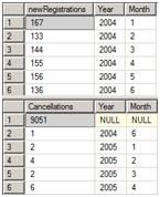
Figure 2: The counts of new registrations and cancellations.

Let’s manually calculate the first few results. The first month, January, 2004, has 167 new subscriptions with no cancellations; therefore, the running total is 167. There are no cancellations until June 2004, so we can just add the new subscriptions for each month through May. In June, we have to subtract one cancellation. Table 1 shows the results for the first few months of 2004, manually calculated, which provide a good representation of the report.

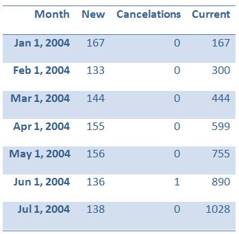
Table 1: The report for 2004

Now we have a means to validate the results returned by our report, we’re ready to start building it. Remember that, just like Peso, we are unlikely to come up with the best solution first; more likely we’ll create a workable solution first and then tweak it to improve performance. Of course, after each tweak of your own solutions, be sure to implement regression testing to make sure that the improved solution still returns the correct results.

Row by Agonizing Row

The reason that so much SQL code found out in the wilds performs poorly is that SQL is nobody’s “first language” (with the possible exception of Joe Celko). Developers tend to master the basic SQL syntax quickly, but then start firing out SQL data retrieval code in a manner strongly influenced by the philosophy and practices of their primary, procedural programming language. When speaking at my local VB.NET group, I found that some of the developers in the audience were shocked that there is another, better way to perform updates than one row at a time.

At its most brutal, the row-by-row solution might look something like the one shown in Listing 2. There is no aggregation going on at all. What we have here is basically an explicit cursor that runs through every single row in the dataset, one at a time, performing the necessary calculations and keeping track of the running totals in a temporary table.

Listing 2: The RBAR solution

The term row-by-agonizing row (RBAR), first coined by Jeff Moden on SQLServerCentral.com, is apt here. This solution, while providing the correct results, runs in 7 seconds on 10,000 rows, on the hardware used to test the solutions in the contest. When applied to the 1 million row dataset, it took 13 minutes!

Imagine a box of marbles sitting in a box on a table. If you needed to move all the marbles to another box on the other side of the room without picking up either box, how would you do it? Would you pick up each marble, one at a time and march it across the room to the second box? Unless you were getting paid by the minute, you would probably scoop them all up and carry them all in one trip. You would avoid the marble-by-marble method, if you wanted to be efficient.

Faster, but Still Iterative

A kinder, though still iterative solution might take the following approach:

• Create a temporary table (#subscriptions), load it with the DateJoined data from the Registrations table, and then aggregate on this column, by month and year, to get a count of the number of people who joined in each month
• Create a CTE (cancellations), load it with the DateLeft data from the Registrations table, and then aggregate on this column by month and year to get a count of the number of people who left in each month, in each year. In lieu of a CTE, you could also use another temp table or a derived table.
• Update the PeopleLeft column in #subscriptions with the number of people who left in each month, from the CTE
• Use a cursor to loop through each month in the temporary table, calculating the required running total of subscribers

This solution is shown in Listing 3.

Listing 3: The Easy, Iterative Solution

So, instead of looping through every row in the data, we aggregate the data to the month level, and then loop through each possible month in the report performing the calculations. We have a lot of date calculations going on in our INSERT and UPDATE statements. These date calculations are very expensive because multiple functions must operate on each date.

When tested, this solution took 360 milliseconds on 10,000 rows and three seconds on 1 million rows. While still not performing as well as the winning solution, it is a big improvement over the original row-by-row solution.

So, this solution, while still flawed, is at least one that will work adequately on a small report table. The other advantage is that the logic behind it is crystal clear, and it will be an easily maintainable solution. BUT…it doesn’t scale. As the results indicate, as more and more rows are added to the registrations table, the report will take longer and longer to run.

We could spend some time tweaking to improve performance, but let’s move on to an even better way.

The Fastest Solution: DATEDIFF, UNPIVOT, and a “Quirky Update”

The winning script in the competition, script “4e” submitted by Peter Larsson (Peso), is reproduced in Listing 4. As noted earlier, it performs so well that, against 10K rows it is almost un-measurably fast, and even when tested against a dataset of one million rows, it took just milliseconds to run. In other words, Peso’s solution is scalable!

Listing 4 Peso 4e

As you can see, we still have the temporary table and the CTE, but what goes on inside each is quite different. Also, this solution has no need for the dreaded cursor, although it does use a few slightly “unconventional” techniques to arrive at the answer. Let’s break this bad boy apart and see if we can learn something.

The overall strategy behind this solution is to pre-aggregate the data down to the rows required in the report while minimizing the date calculations. By doing so, the query engine makes just one pass through the initial data and works with as little data as possible when calculating the running total.

There are three major sections to the code:

• Aggregation Process– the goal here is to reduce the working dataset, stored in a temp table called #Stage, to the minimum possible number of rows, so that date calculations and the subsequent running total calculation are inexpensive.
• Running Total calculation – here, we run an UPDATE statement on a CTE to calculate the running total
• Producing the report –  making clever use of the OUTPUT clause

The Aggregation Process

The essential goal of this step is the same in Peso’s solution (Listing 4) as it was in the solution seen in Listing 3. We need to build a temp table that contains a row for each month and a count of the new subscriptions and cancellations, upon which to base the running total calculation. However, the way that each solution populates the temp table is very different.

Take a look at the table definition for #Stage table (lines A to B), and you will notice something unusual right away. Whereas in the previous solutions we used a conventional DATETIME type for the theMonth column, Peso uses an integer – more about this later. Go ahead and run the table creation statement (A to B).

The SELECT statement used to populate the table is an aggregate query based on the UNPIVOT operator. Run the SELECT statement without the INSERT (C to I) to see what will actually populate #Stage. Figure 3 shows the partial results. Instead of a date, theMonth contains a number from 1248 to 1316 along with the PeopleJoined and PeopleLeft column totals. The Subscribers column contains zeros at this point. This is the data that will be used in the second part of the solution. Except for having integers in the month, it looks very similar to the spreadsheet we created at the beginning of the article to validate the results.

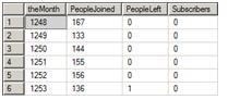
Figure 3: The data used to populate #Stage

Let’s now break this SELECT down, step-by-step to see how it works.

The Pre-aggregation Step

In Listing 3, in order to arrive at a temp table that contained a row for each month and a count of the new subscriptions and cancellations, we had to make two full passes through the Registrations table, once aggregating on the DateJoined column, and once on the DateLeft, performing some expensive date calculations as we went.

Using a “pre-aggregation” involving the DATEDIFF function, followed by a clever trick using the UNPIVOT operator, to normalize the data, Peso managed to take just one pass through the table and so minimize the impact of date manipulations.

In order to understand the final result set shown in Figure 3, we need to first  look at the query that populate the derived table, on which the UNPIVOT operator works. Run lines E to F of Listing 3 will return the contents of this derived table, as shown in Figure 4.

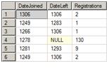
Figure 4: The heart of the unpivoted data

It may be hard to recognize the fact at first glance, but this is, in many respects, the critical moment in the script. In it, we make a single pass through the 10K (or 1 million) row base table, and “summarize” everything we need from it, in order to solve the reporting problem, into only 586 (or 1580) rows. All subsequent operations are performed on this limited working data set and so are relatively inexpensive.

If you look at the original data, you will see that a date can fall anywhere within a month. In order to efficiently eliminate the “day,” this query uses the DATEDIFF function to convert all dates to the number of months that have passed since the date represented by 0 (1900-01-01). So, for example, any date within January 2004 becomes 1248 (104*12). Instead of grouping by month and year, or converting all dates to the first of the month, this solution just converted all the dates to an integer. Eventually, as we perform the running total calculation in the second part of the solution, these integer values are converted back to dates, using DATEADD.

The query counts the number of rows grouped by the DateJoined and DateLeft calculated values. Therefore, all subscribers who joined and left at the same time are grouped together, or “connected”, as part of the pre-aggregation.

You may be wondering why the solution leaves the dates as integers in the INSERT statement and converts them back to dates at the end of the process. It would be simple to just apply a DATEADD function to add the months back in the first statement:

DATEADD(M,DATEDIFF(M,0,DateJoined),0)

This would convert all the dates to the first of the month at one time, but Peso chose to convert them back to dates later, during the running totals calculation. By doing so, the DATEADD function to convert back to date was performed on just 69 values instead of up to 20,000 values (the 10,000 rows times two dates for each row minus the NULLs)

The UNPIVOT Trick

The next step is to “normalize”, or unpivot, the pre-aggregated data. This is the step that means we can avoid any further reads of the base table, because it gives us all the data we need calculate the monthly number of subscribers.

Let’s look at the UNPIVOT part of this statement (F to G), by running the query in Listing 5, which temporarily removes the GROUP BY and HAVING clauses and replaces the SELECT list found in the original solution.

Listing 5: The un-aggregated UNPIVOT query

Figure 5 shows the data after the pre-aggregation together with the unpivoted results:

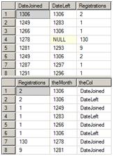
Figure 5: Before and after unpivoting

As you can see, the UNPIVOT operator, introduced with SQL Server 2005, takes column headings and turns them into data. This is the opposite of the PIVOT function that turns data into column headings.

NOTE:
Pre SQL Server 2005, we could have used a derived table with UNION ALL to mimic the UNPIVOT functionality. However, that would have led to two passes on the source table, and not just one.

In this case, the DateJoined and DateLeft column names now become values in the theCol column. The integer values stored in DateJoined and DateLeft become individual entries in a new column, theMonth.  Now, each row contains a number representing the month, a number of registrations, and a value showing whether the data represents a new subscription or a cancellation.

Now we have a list of registrations by month and action (see Figure 6). If you take a closer look at the data after the UNPIVOT is applied, you will see that we have multiple rows for each theMonth and theCol combination. For example, Figure 6 shows two rows for month 1306 and DateLeft. The duplicates exist because the initial aggregation grouped the data on the combination of DateJoined and DateLeft. Since we have split those values apart, there are now duplicates and further aggregation must be done.

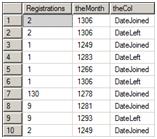
Figure 6: The UNPIVOT results

Repivot and Aggregate

Moving out a bit more, let’s look at how we re-pivot the data and perform the final aggregation. The SELECT list (C to D) creates a sum of PeopleJoined and a sum of PeopleLeft grouped by theMonth (G to H). The code to focus on here is shown in Listing 6.

Listing 6: Using CASE to pivot

The CASE function in the SELECT list determines which rows to count for PeopleJoined and which to count for PeopleLeft. If theCol equals DateJoined, then the row belongs in PeopleJoined. If theCol equals DateLeft, then the row belongs to PeopleLeft. For those of you familiar with the PIVOT function, you probably know that using CASE is another way to pivot data. In this case, the query “pivots” the theCol column to create a total for PeopleJoined and PeopleLeft for each month. Peso could have chosen to use PIVOT instead, but he found that the CASE method was slightly faster. Figure 7 shows how the data looks after pivoting with CASE.

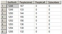
Figure 7: After aggregating

Finally, the HAVING clause (H to I) filters out any rows with no new subscriptions. In the 10,000 rows, all months after September 2009 have cancellations, but no new subscriptions, and future months are not part of the report. Since HAVING filters rows out after aggregates are applied, the CASE function in the WHERE clause returns the total number of new subscriptions after grouping on theMonth. If a month contains only cancellations, as in the months after September 2009, the CASE function returns zero, and the HAVING clause filters those rows out.

We now have 69 rows which is also the number of rows (months) that will appear in the report. For each month (still represented by the integer result of DATEDIFF), we know the number of subscribers and the number of cancellations. The only thing missing is the number of subscriptions, which is still set at zero. Peso has managed to get to this point with only one pass through the data by his masterful pre-aggregation, followed by use of UNPIVOT and CASE.

Go ahead and run lines B to I to populate #Stage.

Calculating the Running Total

The next part of the solution calculates the required running total of subscribers via a “quirky” update command operating on a common table expression (CTE) (lines J to O).

Again, let’s walk through it step-by-step.

Use a Variable to help you Count: no Cursors!

So far, the solution has manipulated our data to get it ready for calculating the running total. Instead of using a while loop or a cursor to calculate this total, a variable @Subscribers is defined and set to zero (I to J). Initializing a variable on the same line that the variable was defined is new to SQL Server 2008. If you are using SQL Server 2005, you will have to change this line:

Into these two lines

Even though we are not using any kind of loop, behind the scenes SQL Server updates one row at a time. Luckily, the pre-aggregation used before getting to this point has transformed the 10,000 original rows into 69, and the implicit cursor that SQL Server uses is faster than an explicit cursor.

The Ordered CTE

CTEs were introduced with SQL Server 2005. At a minimum, you can use CTEs to replace temp tables and views or to separate out a part of the logic of your query. CTEs also have some special uses, for example, for performing recursive queries.

Inside the CTE, we convert back to “normal” dates, and we do this by loading the data from our staging table into a CTE, using the DATEADD function as we go. Since DATEADD is used just once for this small number of rows, it is not that expensive.

If you run just the query inside the CTE definition (K to L), you will see that now theMonth has been converted back into a date and that the data is sorted. Only the running total of subscribers is missing. Figure 8 shows the partial results.

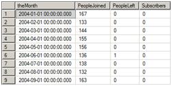
Figure 8: The CTE results

Normally, you cannot order data inside a CTE. One way around this rule is to use the TOP keyword, which allows you to retrieve a number or percentage of rows. In order to control which rows a query returns when using TOP, you can use ORDER BY to sort the data. In this case, Peso chose to use the largest possible integer, 2147483647, to make sure that all the rows will be returned.

The Quirky Update

You can use a CTE in one statement to select, update, delete, or insert data. This is the first time that I have seen the UPDATE statement update the data in the CTE itself (M to N) and not just another table joined to the CTE, though there is nothing stopping you from doing so as long as no rules for updating data are violated.  The statement actually updates the #Stage table, which is the basis for the CTE. The UPDATE statement includes an OUTPUT clause (N to O) which we will discuss shortly.

The SET clause of the UPDATE statement has an interesting formula:

For each row of our data, the Subscribers column is set to the current value of the variable @Subscribers and then increased or decreased based on what happened that month. The value stored in Subscribers, once it is calculated, is saved in the variable. The variable is then available for the next row of data.

This style of update is unofficially referred to as a “quirky update”. It refers to the ability to update variables and columns in a table simultaneously and in an ordered fashion. Here, the ordering is guaranteed by the ORDER BY in our CTE. If this technique were applied to a permanent table the ordering would be established by the table’s clustered index; the update would be done according to the clustered index, but would fail of the table was partitioned, or if parallelism occurred. In any event, it is very important that the calculation is done in the correct order, and that order is guaranteed in this example.

Since the #Stage table is a heap we won’t have problems with the ordering being affected by a clustered index. We won’t get parallelism either because the data is now only 69 records, and holds much less data than a page. Finally, partitioning is not possible on temporary tables.

Producing the Report: A clever use for OUTPUT

The UPDATE statement populates the Subscribers column of the #Stage table. After the update, if we just select the current contents of #Stage, we have the report.  Instead of doing that, Peso chose to use an OUTPUT clause, another relatively new T-SQL feature, introduced with SQL Server 2005. The OUTPUT clause can be used along with any data manipulation statement. It provides deleted and inserted tables, just like triggers do. The deleted table returns the data before the transaction. It can be data that is deleted or the data before it is updated. The inserted table returns the data after the transaction. It can be data that is inserted or data after the update. In this case, the inserted table returns the data how it looks after the update. By using this technique, we avoided accessing the table again to display the data.

Run the last part of the script (I to P) to see that the report works. Figure 9 shows the partial results.

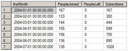
Figure 9: The report

One Small Hole

It was stated as part of the competition rules that it could be assumed that all months had at least one new subscriber.

However, it’s worth noting that if there was a particular month that had no new subscriptions, then that month would not be included in the results. In fact, if a month in the middle of the data had no new subscriptions but had some cancellations, the report will not count the cancellations, and the report will be incorrect. To demonstrate this, change the DateJoined values to 2004-07-01 in the rows where the DateJoined values are within June, 2004 in the Registrations table. Then run the script again. You will see that the report no longer includes the cancellation and all the subsequent values are incorrect.

Fortunately, this problem is easily overcome, via something like an outer join to a sequence or numbers table (see, for example, http://weblogs.sqlteam.com/peterl/archive/2009/11/03/Superfast-sequence-generators.aspx)

Not Quite as Fast, but a Bit More Conventional

Not all queries and scripts require that you take the time to tune them to be fastest they can possibly be. The performance of a query that runs once a month does not matter as much as a query that runs 1000 times a minute. Of course, as you learn more, you will automatically incorporate better performing techniques into your code.

In the real world, there is a balance to be struck between maintainability and outright speed. However, once you’ve started to understand the considerations that are involved in getting the code to run as fast as possible, you can then decide to “back out” to what might be a slightly slower but more maintainable solution. Alternatively, you might decide that the time required to get the code as fast as possible is more time than you have to spend.

So, for example, if we had established Peter’s solution (Listing 4) as the fastest, but felt that we were willing to sacrifice some of the speed in return for ease of understanding and maintainability, then we might opt for a compromise solution, such as that shown in Listing 7. It is based on the “faster but still iterative” solution from Listing 3, but borrows Peso’s DATEDIFF technique to reduce the number of required date calculations.

Listing 7: The compromise solution

When this “compromise” solution was tested, it ran in 74 ms against 10,000 rows and in 847 ms against 1 million rows. Still quite a bit slower than Peso’s solution, but not bad! Even though it uses a cursor for the running the total calculations, the population of the temp table has been improved, and the performance is acceptable.

The important point to remember is that, really, it is the aggregation process that is the most critical. Once you are working with a small data set, the exact manner in which the running total calculation is performed becomes less of an issue, although it will obviously still have some impact.

Table 2 shows how the four solutions stack up:

Solution	10,000 Rows	1 Million Rows
Row-by-row (Listing 2)	7 seconds	13 minutes
Faster but still iterative (Listing 3)	360 milliseconds	3 seconds
Peso  (Listing 4)	0 milliseconds (too fast to measure)	300 milliseconds
Not quite as fast, but conventional (Listing 7)	74 milliseconds	840 milliseconds

Summing Up

The real proof of performance to Peso’s brilliant solution is that, even when Phil Factor tested it against one million rows, the report ran in milliseconds. Here are some of the important points:

• Avoid row-by-row processing, unless on just a handful of rows
• Pass through the data as few times as possible, preferably just once
• Use DATEDIFF to convert the date to an integer if the day of the month is not needed
• Minimize calculations whenever possible by pre-aggregating to a small number of rows first
• Use UNPIVOT and CASE to realign the columns
• Use a variable, instead of a cursor, to calculate running totals
• The OUTPUT clause can be used to display data during an update instead of running an additional SELECT statement

At the very least, I hope you have learned that there can be many ways to come up with the correct answer, but not all solutions are created equal.

The fastest solution presented in this article has reached perfection in terms of performance and scalability. Is it always worth attempting to achieve perfection? Even the SQL Server query optimizer comes up with a plan that is “good enough” and not necessarily perfect. But some techniques perform so poorly on large datasets that learning how to avoid them will pay tremendous dividends.