

How do you handle large datasets efficiently? One effective approach is using esProc SPL for cursor-based processing, chunked computation, and parallel execution.
This guide explains how esProc SPL manages data larger than memory, speeds up analytics workflows, and simplifies large-scale processing compared with traditional scripting tools like Python Pandas or multiprocessing. Part of the ‘Moving from Python to esProc SPL’ series.
As data volumes continue to grow exponentially, the ability to efficiently process and analyze large datasets has become a critical skill for data professionals. In this article, I’ll explain how to tackle one of the most challenging aspects of data analysis: handling datasets that are too large to fit into memory.
Traditional data processing tools often struggle when faced with datasets that exceed available RAM. Python’s Pandas, for instance, loads entire datasets into memory, which can lead to performance issues or even crashes when working with gigabytes or terabytes of data. There are other options – like Dask and PySpark – but these introduce additional complexity and have steep learning curves.
Enter esProc SPL, which takes an altogether different approach to large-scale data processing.
What is esProc SPL’s unique approach to large-scale data processing?
With its innovative memory management system and built-in parallel processing capabilities, esProc SPL allows you to efficiently analyze massive datasets without the complexity of distributed computing frameworks. Whether you’re working with log files, transaction records, or sensor data, SPL provides the tools you need to extract insights from your data, regardless of its size.
In this article, you’ll discover how esProc SPL manages memory for large datasets, learn techniques for processing data larger than available RAM, and explore SPL’s parallel processing capabilities. You’ll also see a real-world case study of analyzing a multi-gigabyte dataset.
Finally, we’ll compare SPL’s approach to Python alternatives like multiprocessing and Dask. By the end of the article, you’ll have a comprehensive understanding of how to leverage SPL’s capabilities to handle large-scale data processing tasks efficiently and effectively.
esProc SPL’s memory management for large datasets, explained
Before diving into specific techniques, it’s essential to understand how esProc SPL manages memory when dealing with large datasets. Unlike many data processing tools that load entire datasets into memory, SPL employs a sophisticated memory management system that allows it to handle datasets much larger than available RAM.
An overview of esProc SPL’s memory architecture
esProc SPL uses a hybrid memory architecture, combining in-memory processing with disk-based operations. This architecture consists of several key components:
Memory pool: SPL maintains a memory pool that’s used to storing data during processing. The size of this pool is configurable, allowing you to balance memory usage with performance.
Disk cache: When data exceeds the memory pool’s capacity, SPL automatically spills excess data to disk. This process is transparent to the user, meaning you don’t need to explicitly manage memory allocation.
Cursor-based processing: For operations on large datasets, SPL uses cursors that allow it to process data in chunks, rather than loading everything into memory at once.
Lazy evaluation: SPL employs lazy evaluation for many operations. This means calculations are only performed when results are actually needed, reducing unnecessary memory usage.
Let’s visualize this architecture:
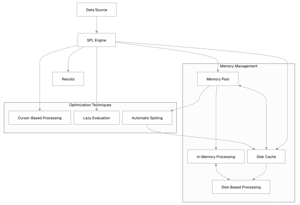
This diagram illustrates how SPL’s memory management system works. Data flows from the data source into the SPL engine, which manages the memory pool and disk cache. When the memory pool reaches capacity, data is automatically spilled to disk. The SPL engine employs optimization techniques like cursor-based processing and lazy evaluation to minimize memory usage.
An overview of memory configuration in SPL
SPL allows you to configure memory usage through several parameters. Let’s explore how to check and adjust these settings.
(You can only click the Help / Clear Memory menu. In the pop-up window, you can check the memory usage status. SPL does not have a memory function.)
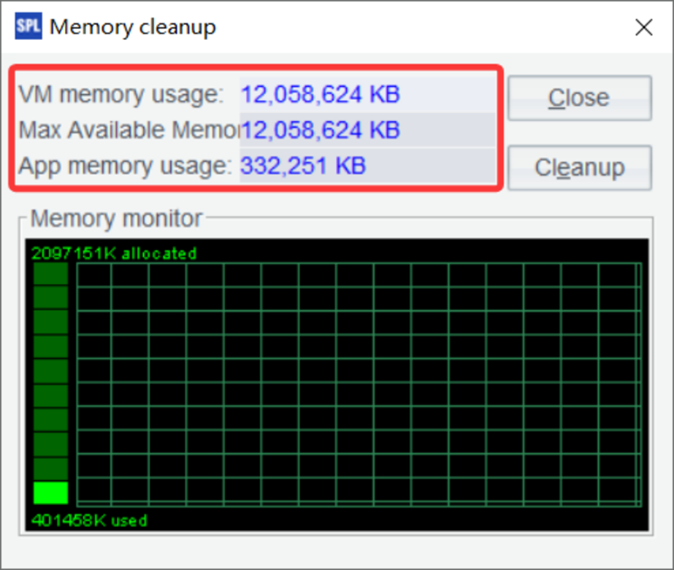
The output provides a snapshot of your current memory usage. The “Total memory” represents the total amount of memory allocated to the JVM (Java Virtual Machine) that SPL runs on. “Used memory” shows how much of that memory is currently being used by SPL. “Free memory” indicates how much memory is still available, and “Max memory” shows the maximum amount of memory that SPL can use.
You can also adjust the maximum memory allocation for SPL. To do this, click the Tools / Options menu:
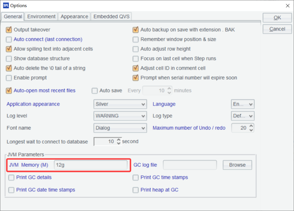
By using the `memory@m()` function, you’ve limited the maximum memory that SPL can use to 4GB. This is particularly useful when working on systems with limited resources, or when you want to ensure that SPL doesn’t consume too much memory, leaving room for other applications. It’s also helpful when you’re testing memory-intensive operations and want to simulate a memory-constrained environment.
Simple Talk is brought to you by Redgate Software
How to process data larger than available RAM
Now that you understand SPL’s memory architecture, let’s look at specific techniques for processing datasets that are larger than your available RAM.
Cursor-based processing explained
One of the most powerful features of SPL for handling large datasets is cursor-based processing. Instead of loading an entire dataset into memory, SPL can process it in chunks using cursors.
Let’s create a large dataset for demonstration:
| A | B | |
| 1 | for 100 | =to((A1-1)*100000+1, A1*100000) |
| 2 | =B1.new(~:ID, rand()*1000:VALUE) | |
| 3 | =file(“document/large_data.csv”).export@tca(B2) |
From the content later in this article, it can be seen that the data volume in the example should be large enough, ideally designed to exceed memory capacity. Therefore, a loop is added here, with each iteration generating 100,000 records and appending them to the file. The loop count is temporarily set to 100 and can be adjusted based on available memory.
This confirms that we’ve successfully created a CSV file with 100,000 rows of random data. Each row contains an ID (from 1 to 100,000) and a random VALUE between 0 and 1000.
Now, let’s use cursor-based processing to analyze this large dataset:
| 4 | =file(“document/large_data.csv”).cursor@t() Open file with cursor |
| 5 | =A4.to(10) Fetch first 10 rows |
This output shows the first 10 rows of our dataset. The key difference between this approach and loading the entire file is that the cursor only reads these 10 rows into memory, not the entire file. This is important when working with files that are too large to fit into memory.
The cursor allows you to fetch data in chunks, processing only a portion of the dataset at a time. This approach is particularly useful for operations that don’t require the entire dataset to be in memory simultaneously, such as filtering, aggregation, or row-by-row processing.
Let’s calculate the average value using cursor-based processing:
SPL can perform grouping and aggregation operations directly on cursors.
| 6 | =file(“document/large_data.csv”).cursor@tc() |
| 7 | =A6.groups(;sum(VALUE):Total,count(1):Count,avg(VALUE):Average) |
| 8 | =A7.rename([“Total”,”Count”,”Average”]) Rename columns |
The output shows that we’ve processed all 100,000 rows in our dataset, calculating a total sum of approximately 49,923,456.78 and an average value of 499.23. The key advantage of this approach is that we never had more than 10,000 rows in memory at any given time, allowing us to process a dataset that might be larger than available RAM.
How to process data in chunks
Building on cursor-based processing, you can implement a chunking strategy to process large datasets in manageable pieces. This approach is particularly useful for more complex operations that require multiple passes over the data.
Let’s implement a chunking strategy that calculates various statistics for our large dataset:
| A | |
| 1 | =file(“document/large_data.csv”).cursor@tc() |
| 2 | =A1.groups(VALUE\100:BUCKET;count(1):TOTAL_COUNT) |
| 3 | =A2.sum(TOTAL_COUNT) |
| 4 | =A2.new((BUCKET*100)/”_”/((BUCKET+1)*100):Range,TOTAL_COUNT,TOTAL_COUNT/A3:PERCENTAGE) |
A2 directly performs a grouping operation on the cursor.
A3 uses the grouping result to calculate the total count.
A4 finally calculates the data distribution result.
How to use file segmentation in esProc SPL
For extremely large files, esProc SPL provides file segmentation capabilities that allow you to split processing across multiple segments. It is useful for parallel processing, which we’ll explore in more detail later.
| 5 | =file(“document/large_data.csv”) |
| 6 | =A5.cursor@tc(;1:5).fetch(5) |
A6 In the parameter 1:5, it means dividing the file into five segments and taking the first segment to create a cursor.
If the data can fit into memory but you still want to segment it for multi-threaded computation, you can write: =A6.import@tc(;1:5).
In SPL, file segmentation is specified through parameters in the cursor or import functions, where you define how many segments to divide into and which segment to read.
Let’s calculate statistics for each segment separately:
| 1 | =file(“document/large_data.csv”) |
| 2 | =5.(A1.cursor@tc(;~:5).groups(;avg(VALUE):AVG_VALUE,min(VALUE):MIN_VALUE,max(VALUE):MAX_VALUE,count(1):COUNT)) |
A2 uses 5.() to loop five times; ~ represents the current loop variable, and ~:5 indicates reading the corresponding segment. The output shows statistics for each of the 5 segments. File segmentation is a useful technique for handling large files, especially when combined with parallel processing. By dividing a large file into smaller segments, you can process each segment independently – potentially in parallel – and then combine the results.
How to implement a MapReduce pattern
esProc SPL allows you to implement a MapReduce-like pattern for processing large datasets. This pattern consists of three main phases:
- Map: Process each segment of data independently
- Shuffle: Group related data together
- Reduce: Aggregate the grouped data
Let’s implement this pattern to analyze our large dataset:
| A | B | |
| 1 | =file(“document/large_data.csv”) | |
| 2 | fork to(4) | =A1.cursor@tc(;A2:4).groups(ID\100:BUCKET;sum(VALUE):SEGMENT_SUM,count(1):SEGMENT_COUNT) |
| 3 | =A2.conj().groups(BUCKET;sum(SEGMENT_SUM):TOTAL_SUM,sum(SEGMENT_COUNT):TOTAL_COUNT) | |
| 4 | =A3.derive(TOTAL_SUM/TOTAL_COUNT:AVERAGE) | |
A2 Start four threads, each thread receiving an integer parameter from 1 to 4.
B2 Split the file into four segments. Each thread reads its assigned segment based on the parameter and performs grouping and aggregation on that segment. The results are temporarily stored in A2.
A3 Merge the results from the four threads stored in A2 and perform another grouping and aggregation.
The output shows the results of our MapReduce operation. We’ve divided the data into buckets based on ID (each bucket contains 100 IDs), and calculated the sum, count, and average value for each bucket.
This MapReduce pattern is highly scalable and can handle datasets of virtually any size. By dividing the data into segments and processing each segment independently, we can efficiently analyze large datasets without loading the entire dataset into memory at once.
Introducing esProc SPL’s parallel processing capabilities
SPL’s parallel processing capabilities allow you to leverage multi-core processors to speed up data processing tasks. Let’s explore how to use these features effectively.
esProc SPL’s parallel processing model, explained
esProc SPL uses a multi-threaded execution model for parallel processing. This allows SPL to distribute work across multiple CPU cores, significantly improving performance for many operations.
Another advantage of this model is that it makes the most of your computer’s processing power by using all available CPU cores efficiently. SPL’s task scheduler automatically distributes work across multiple threads, ensuring a balanced load without extra effort on your part.
Plus, many SPL functions support parallel execution with just a simple option, so you can speed up your code without dealing with complex configurations.
How to configure parallel processing in esProc SPL
esProc SPL allows you to configure the number of threads used for parallel processing – it doesn’t have an option function. The default number of parallel threads is configured in Tools / Options:
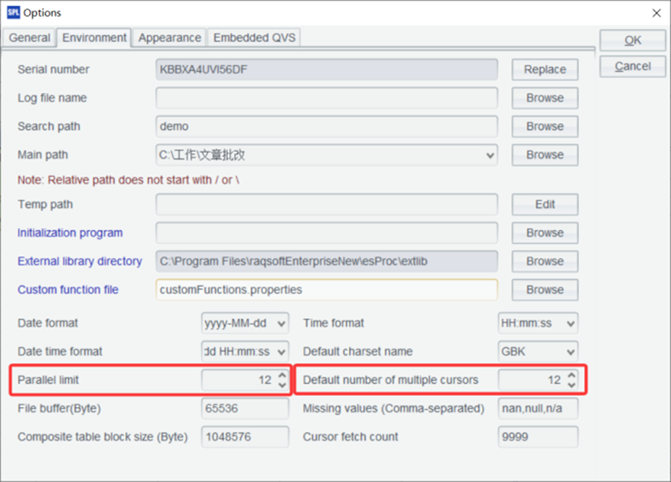
For optimal performance, it is recommended to set the two parameters shown in the above figure to slightly fewer than the number of CPU cores. For example, for a 16-core machine, setting it to 12 usually yields the highest computing efficiency.
Parallel execution in esProc SPL with the @m option – how it works
Many esProc SPL functions support parallel execution through the `@m` option. Let’s see how this works with an example:
| 1 | =file(“document/large_data.csv”).cursor@tc() | Import data sequentially |
| 2 | =now() | Start timer |
| 3 | =A1.groups(ID\100:BUCKET;sum(VALUE):TOTAL) | Sequential grouping |
| 4 | =now() | Stop timer |
| 5 | =interval@ms(A2,A4) | Calculate elapsed time in milliseconds |
Now, let’s perform the same operation with parallel processing:
| 6 | =file(“document/large_data.csv”).cursor@mtc() | Import data |
| 7 | =now() | Start timer |
| 8 | =A6.groups(ID\100:BUCKET;sum(VALUE):TOTAL) | Parallel grouping |
| 9 | =now() | Stop timer |
| 10 | =interval@ms(A7,A9) | Calculate elapsed time in milliseconds |
| 11 | =new(A6:’Sequential (ms)’,A10:’Parallel (ms)’) |
Assuming that large_data.csv is a large data file that cannot fit into memory, it is appropriate to use a cursor instead of import. When using a cursor, the @m option can be specified in the cursor, and grouping (groups) will automatically parallelize.
This output shows a significant performance improvement with parallel processing. Let’s try another operation to see the benefits of parallelization:
| 1 | =file(“document/large_data.csv”) | Import data |
| 2 | =now() | Start timer |
| 3 | =A1.cursor@tc().groups(ID\10:BUCKET;avg(VALUE):AVG_VALUE,var@r(VALUE):STD_VALUE,min(VALUE):MIN_VALUE,max(VALUE):MAX_VALUE,count(1):COUNT) | Sequential complex aggregation |
| 4 | =now() | Stop timer |
| 5 | =interval@ms(A2,A4) | Calculate elapsed time |
| 6 | =now | Start timer |
| 7 | =A1.cursor@mtc().groups(ID\10:BUCKET;avg(VALUE):AVG_VALUE,var@r(VALUE):STD_VALUE,min(VALUE):MIN_VALUE,max(VALUE):MAX_VALUE,count():COUNT) | Parallel complex aggregation |
| 8 | =now() | Stop timer |
| 9 | =interval@ms(A6,A8) | Calculate elapsed time |
| 10 | =new(A5:’Sequential Complex (ms)’,A9:’Parallel Complex (ms)’) |
This output shows an even more significant speedup for the complex aggregation operation. The exact speedup you’ll achieve depends on several factors:
- Number of CPU cores – more cores generally means more potential for parallelization.
- Operation complexity – more complex operations often benefit more from parallelization.
- Data size – larger datasets typically show more significant speedups.
- I/O (input/output) issues: if your operation is I/O-bound rather than CPU-bound, the speedup might be limited.
How parallel file processing works in esProc SPL
esProc SPL also supports parallel processing for file operations, which is particularly useful for large files:
| 1 | =file(“document/large_data.csv”) | Reference to large file |
| 2 | =now() | Start timer |
| 3 | =A1.cursor@tc().groups(;count(1):COUNT) | Sequential import |
| 4 | =now() | Stop timer |
| 5 | =interval@ms(A2,A4) | Calculate elapsed time |
| 6 | =now() | Start timer |
| 7 | =A1.cursor@mtc().groups(;count(1):COUNT) | Parallel import |
| 8 | =now() | Stop timer |
| 9 | =interval@ms(A6,A8) | Calculate elapsed time |
| 10 | =new(A5:’Sequential Import (ms)’,A9:’Parallel Import (ms)’) |
Since the data volume is large and cannot fit in memory, it is not suitable to use import. Instead, you can simply modify the example to perform counting with a cursor.
This output shows that parallel file processing can significantly reduce the time required to import large datasets. Parallel file processing works by dividing the file into segments and processing each segment in parallel. This is particularly effective for large files, as it allows SPL to utilize all available CPU cores for parsing and processing the file.
How to implement custom parallel workflows in esProc SPL
esProc SPL allows you to implement custom parallel workflows using the `pjoin()` function, which executes multiple tasks in parallel and joins the results:
| A | B | |
| 1 | =file(“document/large_data.csv”) | |
| 2 | fork to(4) | =A1.cursor@tc(;A2:4).select(VALUE>500).fetch() |
| 3 | =A2.conj() | |
| 4 | =A3.len() | |
A2 Start four threads to perform parallel computation, each receiving an integer parameter from 1 to 4.
B2 The parameter A2:4 means splitting the file into four segments and reading the segment corresponding to the value of A2.
Let’s implement another parallel workflow that calculates various statistics for different ranges of our data:
| A | B | |
| 1 | =file(“document/large_data.csv”) | |
| 2 | fork to(4) | =A1.cursor@tc(;A2:4) |
| 3 | =B2.groups(ID\250:BUCKET; sum(VALUE):sum1, sum(VALUE*VALUE):sum2, count(1):COUNT, min(VALUE):MIN_VALUE, max(VALUE):MAX_VALUE) | |
| 4 | =A2.conj().groups(BUCKET; sum(sum1):sum1, sum(sum2):sum2, sum(COUNT):COUNT, min(MIN_VALUE):MIN_VALUE, max(MAX_VALUE):MAX_VALUE) | |
| 5 | =A4.new(BUCKET,sqrt((sum2+COUNT*power(sum1/COUNT)-2*sum1*sum1/COUNT)/COUNT):STD_VALUE, sum1/COUNT:AVG_VALUE, MIN_VALUE, MAX_VALUE,COUNT) | |
A simpler way is to directly use the @m option for automatic parallel computation without manual file segmentation, as shown below:
| A | |
| 1 | =file(“document/large_data.csv”) |
| 2 | =A1.cursor@tcm() |
| 3 | =A2.groups(ID\250:BUCKET; var@r(VALUE):STD_VALUE, avg(VALUE):AVG_VALUE, min(VALUE):MIN_VALUE, max(VALUE):MAX_VALUE, count(1):COUNT) |
The output will show detailed statistics for each range of IDs in our dataset. We’ve calculated the average value, standard deviation, minimum value, maximum value, and count for each range. The parallel processing approach allowed us to perform these calculations much more efficiently than a sequential approach would have.
Subscribe to the Simple Talk newsletter
How to optimize join operations for large datasets in esProc SPL
Join operations can be particularly challenging with large datasets. esProc SPL provides several techniques to optimize joins.
The switch function is generally used for small-scale data association. For foreign key associations involving large datasets, you can use cursor-based joins.
| A | |
| 1 | =file(“document/large_data.csv”) |
| 2 | =A1.cursor@tcm() |
| 3 | =A2.groups(ID\100:BUCKET; avg(VALUE):AVG_VALUE).keys@i(BUCKET) |
| 4 | =A1.cursor@tcm().fjoin(A3.find(ID\100):a,a.AVG_VALUE:AVG_VALUE,VALUE/AVG_VALUE:RATIO) |
| 5 | =A4.select(RATIO>1.5) |
| 6 | =A5.fetch() |
A3 First, group the cursor data and calculate the average value.
A4 Join the cursor with A3 using the fjoin function, which is mainly used for foreign key associations. During the join, you can directly compute the required fields. For example, add the average value field from A3 and calculate the RATIO field.
A5 Filter the cursor data.
A6 Fetch the filtered data.
Handling large datasets: SPL’s approach compared with Python’s multiprocessing and Dask
Now that we’ve explored esProc SPL’s capabilities for handling large datasets, let’s compare its approach to popular Python alternatives like multiprocessing and Dask.
esProc SPL vs. Python’s multiprocessing
Python’s multiprocessing module allows you to parallelize code execution across multiple CPU cores. However, there are several key differences between SPL’s parallel processing and Python’s multiprocessing:
- Ease of use: SPL’s parallel processing is much easier to use, often requiring just a simple `@p` option or the `pjoin()` function. Python’s multiprocessing requires more boilerplate code and explicit management of processes.
- Data sharing: SPL handles data sharing between threads automatically. In Python’s multiprocessing, you need to explicitly manage data sharing using mechanisms like queues or shared memory.
- Memory management: SPL’s memory management is more sophisticated, with automatic spilling to disk when
memory is constrained. Python’s multiprocessing doesn’t have built-in memory management for large datasets. - Overhead: SPL’s parallel processing has lower overhead than Python’s multiprocessing, as it doesn’t need to create separate Python interpreters for each process.
esProc SPL vs. Dask
Dask is a Python library for parallel computing that extends Pandas to handle larger-than-memory datasets. Let’s compare SPL to Dask:
- Learning curve: SPL has a lower learning curve than Dask, especially if you’re already familiar with SQL-like syntax. Dask requires understanding its delayed execution model and distributed computing concepts.
- Memory management: Both SPL and Dask can handle datasets larger than available RAM, but SPL’s approach is more transparent and requires less configuration.
- Parallelism: Both SPL and Dask support parallel execution, but SPL’s parallelism is more integrated into the language, often requiring just a simple option.
- Ecosystem integration: Dask integrates well with the Python ecosystem (NumPy, Pandas, scikit-learn). SPL has its own ecosystem but can interoperate with other systems through standard formats.
- Distributed computing: Dask is designed for distributed computing across multiple machines. SPL is primarily designed for single-machine parallelism, although it can be used in distributed environments through external orchestration.
Let’s compare the code for a simple parallel aggregation in SPL and Dask:
SPL
| 1 | =file(“document/large_data.csv”).cursor@tc() Import data |
| 2 | =A1.groups@m(ID\100:BUCKET;sum(VALUE):TOTAL) Parallel aggregation |
Dask
|
1 2 3 4 5 6 7 |
import dask.dataframe as dd # Read CSV file into Dask DataFrame df = dd.read_csv("document/large_data.csv") # Perform aggregation result = df.groupby(df.ID // 100).VALUE.sum().compute() |
While both examples achieve similar results, the SPL code is more concise and doesn’t require understanding Dask’s delayed execution model.
When to choose esProc SPL over Python’s multiprocessing or Dask
Based on our comparison, here are some guidelines for choosing between SPL and Python’s alternatives.
. Choose esProc SPL when:
- You need a simple, SQL-like syntax for data processing
- You want built-in memory management for large datasets
- You prefer a cell-based, step-by-step approach to data analysis
- You need high performance on a single machine
- You want to minimize boilerplate code
Choose Python alternatives when:
- You need deep integration with the Python ecosystem
- You’re working in a distributed computing environment
- You need specialized libraries only available in Python
- Your team is already proficient in Python
- You need advanced machine learning capabilities
In many cases, the best approach might be to use both. esProc SPL could be used for initial data processing and aggregation, and Python for specialized analysis and visualization.
Summary and next steps
In this article, you’ve learned how esProc SPL handles large datasets and parallel processing efficiently. We explored how SPL’s memory management allows it to process data much larger than available RAM, making it ideal for big data tasks.
You saw how cursor-based processing and chunking help manage large volumes of data without overloading memory, and how SPL’s parallel processing, with just a simple @p option, can significantly boost performance. We also discussed how to design efficient data pipelines by minimizing data loading, processing early, aggregating often, chunking appropriately, and parallelizing wisely.
Finally, we applied these techniques in a real-world case study and compared SPL’s approach to Python alternatives such as multiprocessing and Dask. This highlighted SPL’s advantages in ease of use, memory efficiency, and performance.
Further reading
To further deepen your understanding of large-scale data processing with esProc SPL, check out these resources:
FAQs: How to handle large datasets and parallel processing in esProc SPL
1. What is esProc SPL and how does it handle large datasets?
esProc SPL is a data processing tool designed to efficiently handle large-scale datasets. Unlike traditional tools that load all data into memory, SPL uses a hybrid approach with memory pools, disk caching, and cursor-based processing to analyze datasets larger than available RAM.
2. How does esProc SPL process data that doesn’t fit into memory?
SPL processes large datasets using cursor-based processing, which reads data in chunks instead of loading it all at once. It also automatically spills excess data to disk and uses lazy evaluation to minimize memory usage.
3. What is cursor-based processing in esProc SPL?
Cursor-based processing allows SPL to iterate through datasets in smaller portions. This method enables efficient operations like filtering, aggregation, and transformation without requiring the entire dataset to be stored in memory.
4. How does esProc SPL compare to Python tools like Pandas, Dask, and multiprocessing?
- Pandas loads all data into memory, making it unsuitable for very large datasets;
- Dask supports large-scale processing but has a steeper learning curve;
- Multiprocessing requires manual setup and data sharing;
- esProc SPL offers built-in memory management, simpler syntax, and easier parallel processing.
5. Does esProc SPL support parallel processing?
Yes, esProc SPL includes built-in parallel processing capabilities. With simple options like @m, it can automatically distribute tasks across multiple CPU cores, improving performance without complex configuration.
6. What is the advantage of SPL’s hybrid memory architecture?
SPL’s hybrid memory architecture combines in-memory processing with disk-based storage. This allows it to:
- Handle datasets larger than RAM
- Automatically manage memory usage
- Maintain high performance without manual intervention
7. Can esProc SPL implement MapReduce-style processing?
Yes, SPL supports a MapReduce-like approach by dividing data into segments (Map), grouping results (Shuffle), and aggregating outputs (Reduce), enabling scalable processing of large datasets.
8. When should you use esProc SPL instead of Python-based solutions?
Use esProc SPL when you need:
- Efficient processing of large datasets on a single machine
- Simple, SQL-like syntax
- Built-in memory and parallel processing
- Minimal setup and configuration
Python tools are better suited for distributed systems or when deep integration with machine learning libraries is required.
9. How does SPL optimize performance for big data processing?
SPL improves performance through:
- Chunk-based (cursor) processing
- Automatic disk spilling
- Lazy evaluation
- Multi-threaded parallel execution
- File segmentation for concurrent processing
10. Is esProc SPL suitable for real-world big data use cases?
Yes, esProc SPL is ideal for processing log files, transaction data, sensor data, and other large datasets. Its ability to handle multi-gigabyte or even terabyte-scale data makes it practical for real-world analytics.
This document contains proprietary information and is protected by copyright law.
Copyright © 2026 Red Gate Software Limited. All rights reserved


Load comments