

In the previous article of this “Moving from Python to esProc SPL” series, I covered how to set up esProc SPL and load your first datasets. It’s now time to learn what makes esProc SPL a tool for data analysis: its syntax and data structures. In this article, you’ll learn about SPL’s core syntax elements, its primary data structure (the table), and how to perform common data operations. By the end, you’ll understand how to write effective SPL code and how it compares to equivalent operations in Python.
esProc SPL (Structured Process Language) was designed specifically for data processing, with a syntax that prioritizes readability and efficiency for data operations. If you’re coming from Python, particularly if you’ve used Pandas for data analysis, you’ll find some familiar concepts in SPL and discover approaches that can simplify complex data tasks.
In this article, you’ll learn about SPL’s core syntax elements, its primary data structure (the table), and how to perform common data operations. By the end, you’ll understand how to write effective SPL code and how it compares to equivalent operations in Python.
What is esProc SPL’s syntax, and how does it compare to Python?
esProc SPL’s syntax has a logical flow that will feel familiar if you’re coming from Python, but with some key differences that make it particularly well-suited for data analysis. Let’s look at the basic syntax elements and how they compare to Python.
What is esProc SPL’s basic syntax?
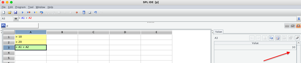
SPL introduces a cell-based structure that enhances readability and debugging. It makes SPL useful for complex data operations, where it is essential to track transformations at each step. SPL organizes code into cells, similar to how a spreadsheet works. Each line of code is assigned to a specific cell (A1, B2, C3, etc.), making it easier to follow the flow of calculations.
| A | ||
| 1 | = 10 | Assign the value 10 to cell A1 |
| 2 | = 20 | Assign the value 20 to cell A2 |
| 3 | = A1 + A2 | Add the values in A1 and A2, store the result in A3 |
When you run this code in the esProc IDE, you’ll see:
This cell-based approach creates a visual flow of your data processing steps. Each cell can be inspected individually. In Python, the equivalent would be:
|
1 2 3 4 |
a1 = 10 a2 = 20 a3 = a1 + a2 print(a3) # Output: 30 |
Python uses a linear, script-based approach, meaning you have to run the entire script to see the results. Unlike SPL’s cell-based execution, Python doesn’t inherently allow you to view intermediate outputs unless you manually print them. SPL supports interactive processing; if you modify and rerun a single cell’s value, only the dependent cells need to be executed again, saving time and computational resources.
What is esProc SPL’s expression syntax?
SPL expressions follow a familiar syntax if you’re coming from Python. You can perform arithmetic operations, string concatenation, and logical comparisons just like in Python.
| A | ||
| 1 | =5+3*2 | Result: 11 |
| 2 | =”Hello”+” World” | Result: “Hello World” |
| 3 | =A1>10 | Result: true |
When you run this code in the esProc IDE (integrated development environment), you’ll see:
A1: 11
A2: Hello World
A3: true
The IDE shows both the expression and its evaluated result, making it easy to understand what’s happening at each step. This is helpful when debugging complex expressions. Python’s equivalents are:
|
1 2 3 4 5 6 7 8 9 10 11 |
# Arithmetic operation: Multiplication happens first, then addition a1 = 5 + (3 * 2) # Result: 11 # String concatenation: Combines "Hello" and " World" a2 = "Hello" + " World" # Result: "Hello World" # Boolean comparison: Checks if a1 is greater than 10 a3 = a1 > 10 # Result: True # Print the results print(a1, a2, a3) |
The main difference is that Python uses `True`/`False` (capitalized) for boolean values, while SPL uses `true`/`false` (lowercase). Also, in Python, you typically need to add print statements to see intermediate results, whereas in SPL, the results are automatically displayed in the IDE.
How does method chaining work in esProc SPL?
Like Python, SPL supports method chaining, allowing you to perform multiple operations in sequence:
| A | ||
| 1 | = file(“sales.csv”).import@ct() | Import CSV file |
| 2 | = A1.select(Amount>1000) .sort(Amount:-1) .to(5) Get top 5 rows | Filter rows Sort by Amount descending Get top 5 rows |
The output will show the top 5 orders with amounts greater than $1000, sorted by amount in descending order. The table format makes it easy to see each record’s OrderID, Customer, Product, Amount, and Date. The Python equivalent, using pandas, would be:
|
1 2 3 4 5 |
import pandas as pd df = pd.read_csv("sales.csv") result = df[df['Amount'] > 1000].sort_values('Amount', ascending=False).head(5) print(result) |
Both SPL and pandas accomplish the same task, but SPL’s syntax is more streamlined. Instead of calling multiple functions separately, SPL allows you to chain them in a way that naturally follows how you think about the data: filter, sort, and retrieve.
Comments and code organization in esProc SPL
In SPL, comments should generally be placed in a separate cell, not mixed with code.
| A | ||
| 1 | = 5 * 10 | Calculate product of 5 and 10 |
| 2 | = A1 / 2 | Divide the result by 2 |
This differs from Python’s `#` comment syntax. SPL also uses indentation to show logical structure in control flows, similar to Python:
| A | |
| 1 | = 15 |
| 2 | = if(A1 > 10, A1*2, A1/2) |
If written as an ‘if’ statement, the table should look like this: [if and else are keywords with no preceding = sign]
| A | B | ||
| 1 | = 15 | ||
| 2 | if A1 > 10 | >A1=A1 * 2 | Double the value if A1 > 10 |
| 3 | else | >A1=A1 / 2 | Halve the value if A1 <= 10 |
The output (A6) would be: 30. Since A1 (15) is greater than 10, the value is doubled to 30.
Simple Talk is brought to you by Redgate Software
How do variables and data types work in esProc SPL?
esProc SPL, like Python, is dynamically typed, meaning you don’t need to declare variable types explicitly. However, understanding the available data types is important for effective data manipulation.
What basic data types are supported in esProc SPL?
SPL supports several basic data types:
| A | |
| 1 | =5 Integer |
| 2 | =5.25 Decimal |
| 3 | =”Hello” String |
| 4 | =true Boolean |
| 5 | =null Null value |
| 6 | =date(“2023-06-15”) Date |
When you run this code in the esProc IDE, you’ll see:
A1: 5
A2: 5.25
A3: Hello
A4: true
A5: null
A6: 2023-06-15
Each cell shows both the assigned value and its data type through visual cues in the IDE. For example, strings are displayed in a different color than numbers, making it easy to identify the type of each value. Strings are left-aligned, underlined, and displayed in black. Numeric values are right-aligned, with integers in blue and doubles in brown. The Python equivalents are:
|
1 2 3 4 5 6 |
a1 = 5 # Integer a2 = 5.25 # Float a3 = "Hello" # String a4 = True # Boolean a5 = None # None value a6 = datetime.date(2023, 6, 15) # Date (requires datetime module) |
One key difference is that SPL has built-in support for date values, while Python requires the datetime module. This makes working with dates more straightforward in SPL, especially for data analysis tasks that often involve date-based calculations.
How does type conversion work in esProc SPL?
SPL provides functions for type conversion:
| A | |
| 1 | =”123″ |
| 2 | =int(A1) Convert string to integer: 123 |
| 3 | =string(A2) Convert integer to string: “123” |
| 4 | =decimal(“45.67”) Convert string to decimal: 45.67 |
| 5 | date(“2023-06-15”) Convert string to date: 2023-06-15 |
When you run this code, you’ll see:
A1: 123 (displayed as a string), A2: 123 (displayed as an integer), A3: 123 (displayed as a string), A4: 45.67 (displayed as a decimal), A5: 2023-06-15 (displayed as a date). The IDE helps you distinguish between different types through visual cues, even when the displayed value looks the same (like the string “123” and the integer 123).
Python’s equivalents are:
|
1 2 3 4 5 6 7 8 9 10 11 12 13 14 15 16 17 18 19 20 21 22 |
import datetime # Define a string containing numeric characters a1 = "123" # Convert string to integer a2 = int(a1) # Result: 123 # Convert integer back to string a3 = str(a2) # Result: "123" # Convert string to floating-point number a4 = float("45.67") # Result: 45.67 # Convert string to date a5 = datetime.datetime.strptime("2023-06-15", "%Y-%m-%d").date() # Result: 2023-06-15 # Print results print(a2, type(a2)) # Output: 123 <class 'int'> print(a3, type(a3)) # Output: 123 <class 'str'> print(a4, type(a4)) # Output: 45.67 <class 'float'> print(a5, type(a5)) # Output: 2023-06-15 <class 'datetime.date'> |
Notice how date conversion in Python requires more code and knowledge of format strings, while SPL’s date function is more straightforward for common date formats.
Comparing esProc SPL’s primary data structure – the table sequence – to Python’s DataFrame
The table sequence is SPL’s primary data structure for handling tabular data, similar to Python’s DataFrame in pandas. However, there are important differences in how they work and are manipulated.
How do you create a table sequence in esProc SPL?
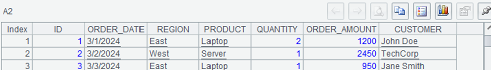
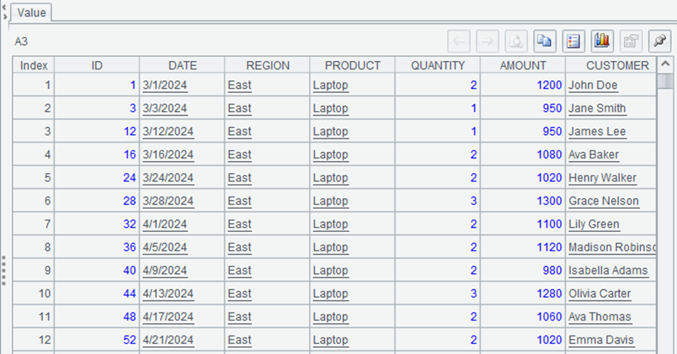
Let’s create a table sequence by importing a CSV file:
| A | ||
| 1 | =file(“document/sales.csv”).import@ct() | Sales data with 100 rows |
| 2 | =A1.to(5) | First 5 rows of the table |
The order of @t and @c does not matter, meaning @ct and @tc are equivalent. If neither the option nor the parameter specifies a delimiter, the default is tab-separated.
If you need to preserve leading zeros or other special formatting, you can use `import@f` to import data as raw strings without parsing:
| A | ||
| 1 | =file(“document/zip_codes.csv”).import@ctf() | ZIP code data with leading zeros preserved |
The Python equivalent is:
|
1 2 3 4 5 6 |
import pandas as pd # Import CSV as DataFrame sales_df = pd.read_csv("sales.csv") # View first 5 rows sales_df.head(5) |
You can also create a table manually:
| A | |
| 1 | =create(DATE, REGION, PRODUCT, AMOUNT, CUSTOMER).record( [date(“2023-04-10”), “East”, “Laptop”, 1250, “TechCorp”, date(“2023-04-15”), “West”, “Monitor”, 450, “HomeOffice”]) |
When defining table structures, field names do not require quotes (more convenient than Python), and inserting records only requires flat collections. The output would be a table with two rows and five columns.
The Python equivalent is:
|
1 2 3 4 5 6 7 8 9 10 11 |
import pandas as pd from datetime import date # Create DataFrame manually sales_df = pd.DataFrame({ "DATE": [date(2023, 4, 10), date(2023, 4, 15)], "REGION": ["East", "West"], "PRODUCT": ["Laptop", "Monitor"], "AMOUNT": [1250, 450], "CUSTOMER": ["TechCorp", "HomeOffice"] }) |
While both table sequences in esProc SPL and DataFrames in Python serve as data structures for handling tabular data, they differ in key aspects. SPL’s table operates in a cell-based environment, where each step is explicitly named and can be referenced later, making it easier to track transformations. In contrast, Python’s pandas DataFrame relies on an object-based approach, where operations are performed directly on the DataFrame object.
Another difference lies in column access: SPL allows you to reference column names directly in expressions, whereas pandas requires bracket notation (df[“column”]) or dot notation (df.column). Additionally, SPL follows a step-by-step execution model, making it easier to debug, while pandas often encourages method chaining, which can be more concise but harder to follow for complex transformations.
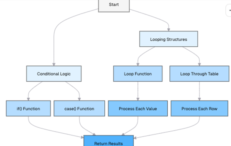
The following flowchart illustrates the parallel workflows in SPL and Python for a typical data processing task, from importing raw data to analysis. While the overall flow is similar, the syntax and approach differ in important ways:
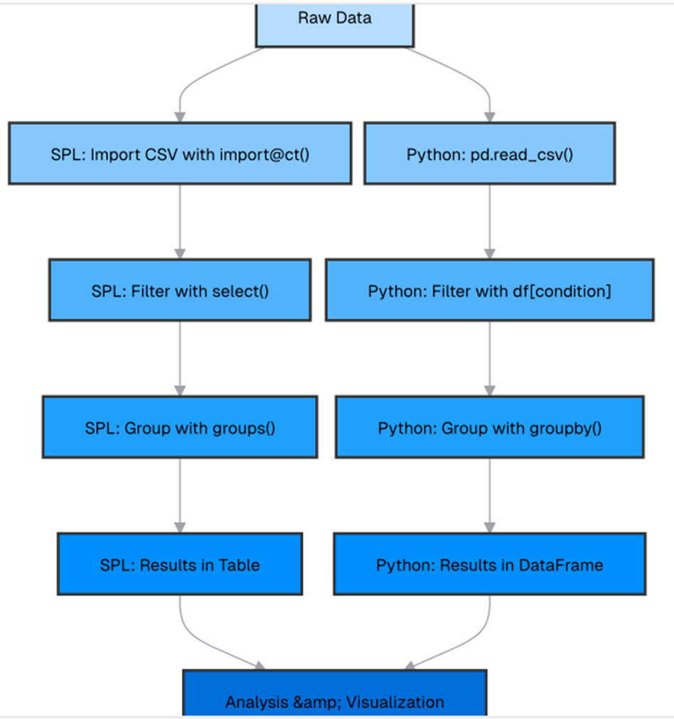
Table properties and methods in esProc SPL
SPL provides various properties and methods to work with tables:
| A | ||
| 1 | =file(“document/sales.csv”).import@ct() | Sales data with 100 rows |
| 2 | =A1.len() | 100 |
| 3 | =A1.fname() [“DATE”, “REGION”, “PRODUCT”, “AMOUNT”, “CUSTOMER”] | |
| 4 | =A1.fname(1) | “DATE” |
| 5 | =A1.AMOUNT | 4 |
The output shows the number of rows, column names, the name of the first column, and the position of the AMOUNT column. These properties are useful for understanding the structure of your data.
The equivalents in Python are:
|
1 2 3 4 5 6 7 8 9 10 11 |
import pandas as pd sales_df = pd.read_csv("sales.csv") # Number of rows row_count = len(sales_df) # Get column names column_names = sales_df.columns.tolist() # Get the name of the first column first_column = sales_df.columns[0] # Get the position of the AMOUNT column amount_position = sales_df.columns.get_loc("AMOUNT") |
How do columns and rows work in esProc SPL?
esProc SPL provides powerful and intuitive ways to manipulate columns and rows in tables.
How do you rename columns in esProc SPL?
| A | ||
| 1 | =file(“document/sales.csv”).import@ct() | Sales data with 100 rows |
| 2 | =A1.rename(DATE:ORDER_DATE, AMOUNT:ORDER_AMOUNT) | Table with renamed columns |
The output of A2 would have columns renamed from DATE to ORDER_DATE and AMOUNT to ORDER_AMOUNT. This is useful when you want to make column names more descriptive or consistent.
The Python equivalent is:
|
1 2 3 4 5 |
import pandas as pd sales_df = pd.read_csv("sales.csv") sales_df = sales_df.rename(columns={"DATE": "ORDER_DATE", "AMOUNT": "ORDER_AMOUNT"}) |
How do you calculate column statistics in esProc SPL?
| A | |
| 1 | =file(“document/sales.csv”).import@ct() |
| 2 | =A1.max(AMOUNT) |
| 3 | =A1.min(AMOUNT) |
| 4 | =A1.avg(AMOUNT) |
| 5 | =A1.sum(AMOUNT) |
The output shows various statistical calculations on the AMOUNT column. These methods provide a quick way to understand the distribution of your data.
The equivalents in Python are:
|
1 2 3 4 5 6 7 8 9 10 11 12 13 14 15 16 |
import pandas as pd # Import the Pandas library # Load the sales dataset from a CSV file sales_df = pd.read_csv("sales.csv") # Calculate the maximum, minimum, average, and total amount from the "AMOUNT" column max_amount = sales_df["AMOUNT"].max() # Get the highest value min_amount = sales_df["AMOUNT"].min() # Get the lowest value avg_amount = sales_df["AMOUNT"].mean() # Get the average value total_amount = sales_df["AMOUNT"].sum() # Get the total sum # Print the results print("Maximum Amount:", max_amount) print("Minimum Amount:", min_amount) print("Average Amount:", avg_amount) print("Total Amount:", total_amount) |
This script reads the sales.csv file, extracts values from the AMOUNT column, and performs basic statistical operations on them.
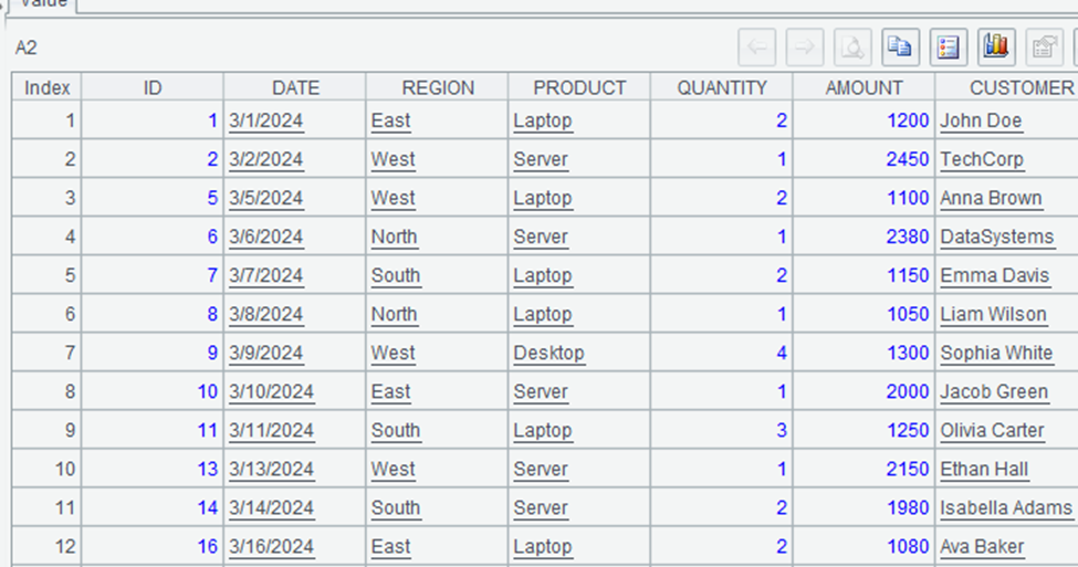
How do you filter rows in esProc SPL?
| A | |
| 1 | =file(“document/sales.csv”).import@ct() |
| 2 | =A1.select(AMOUNT>1000) |
| 3 | =A1.select(REGION==”East” && PRODUCT==”Laptop”) |
The output of A2 would be a table with only rows where AMOUNT > 1000, and A3 would show only rows where REGION is “East” and PRODUCT is “Laptop”. The `select` method is powerful for filtering data based on conditions.
The equivalents in Python are:
|
1 2 3 4 5 6 7 8 9 10 11 12 13 14 |
import pandas as pd # Load the sales data from a CSV file sales_df = pd.read_csv("sales.csv") # Filter rows where the AMOUNT column is greater than 1000 filtered_df1 = sales_df[sales_df["AMOUNT"] > 1000] # Filter rows where the REGION is "East" and the PRODUCT is "Laptop" filtered_df2 = sales_df[(sales_df["REGION"] == "East") & (sales_df["PRODUCT"] == "Laptop")] # Display the filtered data print(filtered_df1) print(filtered_df2) |
How do you sort rows in esProc SPL?
| A | ||
| 1 | =file(“document/sales.csv”).import@ct() | |
| 2 | =A1.sort(AMOUNT) | Table sorted by AMOUNT (ascending) |
| 3 | =A1.sort(AMOUNT:-1) | Table sorted by AMOUNT (descending) |
| 4 | =A1.sort(REGION,AMOUNT:-1) | Table sorted by REGION (asc) then AMOUNT (desc) |
The output of each cell would be the sorted table according to the specified criteria. The `sort` method is flexible, allowing you to sort by multiple columns in different directions.
The equivalents in Python are:
|
1 2 3 4 5 6 7 8 9 10 11 12 13 14 15 16 17 18 19 20 21 22 23 |
import pandas as pd # Import the pandas library # Load the sales data from a CSV file sales_df = pd.read_csv("sales.csv") # Sort the DataFrame by the "AMOUNT" column in ascending order sorted_df1 = sales_df.sort_values(by="AMOUNT") # Sort the DataFrame by the "AMOUNT" column in descending order sorted_df2 = sales_df.sort_values(by="AMOUNT", ascending=False) # Sort the DataFrame first by "REGION" (ascending) and then by "AMOUNT" (descending) sorted_df3 = sales_df.sort_values(by=["REGION", "AMOUNT"], ascending=[True, False]) # Display the sorted DataFrames print("Sorted by AMOUNT (Ascending):") print(sorted_df1) print("\nSorted by AMOUNT (Descending):") print(sorted_df2) print("\nSorted by REGION (Ascending) and AMOUNT (Descending):") print(sorted_df3) |
How do you limit rows in esProc SPL?
| A | ||
| 1 | =file(“document/sales.csv”).import@ct() | |
| 2 | =A1.to(5) | First 5 rows of the table |
| 3 | =A1.sort(AMOUNT:-1).to(5) | five rows with highest AMOUNT values |
The output of A2 would be the first five rows of the table, and A3 would be the five rows with the highest AMOUNT values. The `top` method is useful for limiting the number of rows in your result set.
The equivalents in Python are:
|
1 2 3 4 5 6 7 8 9 10 11 12 13 14 15 16 |
import pandas as pd # Load the sales data from a CSV file sales_df = pd.read_csv("sales.csv") # Retrieve the first 5 rows of the dataset first_5_rows = sales_df.head(5) # Sort the data by the "AMOUNT" column in descending order and get the top 5 entries top_5_by_amount = sales_df.sort_values(by="AMOUNT", ascending=False).head(5) # Display the results print("First 5 rows of the dataset:") print(first_5_rows) print("\nTop 5 rows sorted by AMOUNT in descending order:") print(top_5_by_amount) |
Control structures: loops and conditionals in esProc SPL vs. Python
esProc SPL provides familiar control structures for loops and conditionals, but with some syntax differences compared to Python.
Enjoying this article? Subscribe to the Simple Talk newsletter
How do conditional statements work in esProc SPL?
SPL uses `if` statements similar to many programming languages:
| A | ||
| 1 | =1250 | 1250 |
| 2 | =if(A1>1000,”High”,”Low”) | “High” |
The output shows that since A1 (1250) is greater than 1000, the result is “High.” The `if` function takes three arguments: a condition, a value to return if the condition is true, and a value to return if the condition is false.
Another example:
| A | |
| 1 | =file(“document/sales.csv”).import@ct() |
| 2 | =A1.derive(if(AMOUNT>2000:”Premium”,AMOUNT>1000:”Standard”:”Basic”):CATEGORY) |
The output of A2 would include a new CATEGORY column with values based on the AMOUNT. This is a powerful way to categorize data based on multiple conditions.
The equivalents in Python are:
|
1 2 3 4 5 6 7 8 9 10 11 12 13 14 15 16 17 18 19 20 |
import pandas as pd import numpy as np # Import NumPy for conditional logic # Define a single transaction amount amount = 1250 # Assign category based on amount using a conditional (ternary) operator category = "High" if amount > 1000 else "Low" # Load the sales dataset from a CSV file sales_df = pd.read_csv("sales.csv") # Apply conditional logic to classify sales amounts into categories sales_df["CATEGORY"] = np.where( sales_df["AMOUNT"] > 2000, "Premium", # If amount is greater than 2000, label it as "Premium" np.where(sales_df["AMOUNT"] > 1000, "Standard", "Basic") # Else, categorize into "Standard" or "Basic" ) # Display the first few rows to verify the changes print(sales_df.head()) |
How do loops work in esProc SPL?
esProc SPL provides several ways to implement loops:
How do you implement ‘For Loop’ in esProc SPL?
【Looking at the Python code later, the equivalent SPL code only requires one line and doesn’t need loops.】
| A | |
| 1 | =5.(~*2+1) |
【If using ‘for’, it needs to be written across multiple lines; ‘for’ is a keyword and shouldn’t be preceded by ‘=’.】
| A | B | |
| 1 | =[] | |
| 2 | for 5 | =A2*2 Current value * 2 |
| 3 | =B2+1 B2 + 1 | |
| 4 | >A1=A1|B3 【This sentence is equivalent to Python’s append, and the result is stored in A1.】 |
This loop iterates from 1 to 5, multiplies each value by 2, adds 1, and returns the result. The `for@r` function creates a loop that returns a sequence of values. The `>` symbol indicates that the line is part of the loop body.
The equivalent in Python is:
|
1 2 3 4 5 6 7 8 |
result = [] # Initialize an empty list to store results for i in range(1, 6): # Loop through numbers 1 to 5 value = i * 2 # Multiply the number by 2 value = value + 1 # Add 1 to the result result.append(value) # Append the final value to the list print(result) # Output: [3, 5, 7, 9, 11] |
How do you loop through a table in esProc SPL?
| A | ||
| 1 | =file(“document/sales.csv”).import@ct() | |
| 2 | =A1.select(AMOUNT>1000) | 26 rows where AMOUNT > 1000 |
| 3 | =A2.(CUSTOMER + ” purchased ” + PRODUCT + ” for $” + string(AMOUNT) ) |
This loop function in A3 iterates through the filtered table, creates a formatted string for each row, and adds it to a sequence.
The equivalent in Python is:
|
1 2 3 4 5 6 7 8 9 10 11 12 13 14 15 16 17 |
import pandas as pd # Import the pandas library # Read the sales data from a CSV file into a DataFrame sales_df = pd.read_csv("sales.csv") # Filter rows where the AMOUNT column is greater than 1000 filtered_df = sales_df[sales_df["AMOUNT"] > 1000] # Create a list to store formatted messages result = [ f"{row['CUSTOMER']} purchased {row['PRODUCT']} for ${row['AMOUNT']}" for _, row in filtered_df.iterrows() ] # Print the result for message in result: print(message) |
How does the case function work in esProc SPL?
SPL provides a `case` function for multiple conditions:
| A | |
| 1 | =”Laptop” |
| 2 | =case(A1,”Laptop”:”Electronic”,”Monitor”:”Display”,”Printer”:”Output”,”Unknown”) “Electronic” |
The output shows that since A1 is “Laptop,” the result is “Electronic.” The `case` function takes a value to test, followed by pairs of values and results, with an optional default value at the end.
The equivalent in Python is:
|
1 2 3 4 5 6 7 8 9 10 11 12 |
# Define the product product = "Laptop" # Use a dictionary to map product names to categories category = { "Laptop": "Electronic", "Monitor": "Display", "Printer": "Output" }.get(product, "Unknown") # If product is not found, return "Unknown" # Print the category print(category) # Output: Electronic |
How do functions and procedures work in esProc SPL?
esProc SPL allows you to define custom functions and procedures to encapsulate logic and make your code more modular and reusable.
How do you define functions in esProc SPL?
In SPL, you can define functions using the `function` keyword:
| A | B | |
| 1 | =func Add_number(x,y) | =x+y |
A custom function requires at least two columns and does not need to include ‘return’. This defines a function that adds two numbers. To use this function:
| 2 | =Add_number(5,3) |
The output shows that the function correctly adds 5 and 3 to produce 8. Functions in SPL can take parameters and return values, just like in Python.
The Python equivalent is:
|
1 2 3 4 5 6 7 8 9 |
def add_numbers(x, y): """Returns the sum of two numbers.""" return x + y # Call the function with arguments 5 and 3 result = add_numbers(5, 3) # Print the result print(result) # Output: 8 |
How do functions with tables work in esProc SPL?
Functions can also work with tables:
| A | B | ||
| 1 | =func analyze_sales(ds, min_amount) | =ds.select(AMOUNT>=min_amount) | Filter for amounts >= min_amount |
| 2 | =B1.groups(REGION;count():COUNT,sum(AMOUNT):TOTAL) | Group by region |
This function filters a table for amounts greater than or equal to a minimum value, then groups by region and calculates counts and totals. To use this function:
| 3 | =file(“document/sales.csv”).import@ct() | |
| 4 | =analyze_sales(A4, 1000) | Filtered and grouped sales data |
This example demonstrates how functions can encapsulate complex data processing logic, making your code more modular and reusable.
The Python equivalent is:
|
1 2 3 4 5 6 7 8 9 10 11 12 13 14 15 16 17 18 19 20 21 22 23 24 25 26 27 28 29 30 31 32 |
import pandas as pd # Import the pandas library def analyze_sales(df, min_amount): """ Filters sales data based on a minimum amount and aggregates results by region. Parameters: df (DataFrame): The input sales data. min_amount (int or float): The minimum amount to filter sales. Returns: DataFrame: Aggregated sales data grouped by region. """ # Filter rows where the AMOUNT is greater than or equal to the minimum amount filtered_df = df[df["AMOUNT"] >= min_amount] # Group by REGION and calculate COUNT (number of transactions) and TOTAL (sum of AMOUNT) result = filtered_df.groupby("REGION").agg( COUNT=("AMOUNT", "count"), # Count of transactions TOTAL=("AMOUNT", "sum") # Sum of AMOUNT for each region ).reset_index() # Reset index for a cleaner DataFrame return result # Load sales data from a CSV file sales_df = pd.read_csv("sales.csv") # Analyze sales with a minimum transaction amount of 1000 result = analyze_sales(sales_df, 1000) # Display the result print(result) |
How do lambda functions work in esProc SPL?
SPL also supports lambda functions for concise, inline function definitions:
| A | ||
| 1 | =[1,2,3,4,5] | |
| 2 | =A1.(~*2) | [2,4,6,8,10] |
In SPL, lambda doesn’t require parameter definition – just use ~ directly.
The output shows that each value in the sequence is doubled. The `map` function applies a lambda function to each element of a sequence and returns a new sequence with the results.
The equivalent in Python is:
|
1 2 3 4 5 6 7 8 |
# Define a list of numbers numbers = [1, 2, 3, 4, 5] # Use map with a lambda function to double each number doubled = list(map(lambda x: x * 2, numbers)) # Print the result print(doubled) # Output: [2, 4, 6, 8, 10] |
This code correctly applies the lambda function to each element in the numbers, doubling their values.
esProc SPL error handling and debugging techniques
Effective error handling and debugging are essential skills for any data analyst. esProc SPL provides several techniques for handling errors and debugging your code.
How do you handle errors in esProc SPL?
The correct approach to handle errors in esProc SPL is to use an `if` condition, or check for errors manually. It provides an `error()` function to trigger an error and `string(e)` to capture error messages.
| A | |
| 1 | =if(0!=0,1/0,”Error: Division by zero”) |
The output would be:
A1: Error: Division by zero

The equivalent in Python is:
|
1 2 3 4 5 6 7 |
try: result = 1 / 0 # This will cause a division by zero error message = "Success" # This line will not execute due to the error except Exception as e: message = f"Error: {e}" # Catch the exception and store the error message print(message) # Output: Error: division by zero |
How do you use the debug panel in esProc SPL?
The esProc IDE provides a debug panel that helps you troubleshoot scripts efficiently. You can set breakpoints by clicking in the margin next to the cell where you want execution to pause. Once breakpoints are set, clicking the “Debug” button starts the debugging process. The IDE offers step buttons that allow you to execute the code incrementally, making it easier to identify issues in complex scripts with multiple functions and procedures.
Additionally, the debug panel displays variable values, enabling you to inspect their states at each step. The feature is useful when dealing with intricate calculations or logical conditions, as it allows for a clear understanding of how data changes throughout execution.
How to solve common esProc SPL errors
Here are some common errors you might encounter in SPL and how to solve them:
1. Column Not Found: This occurs when you reference a column that doesn’t exist in your table.
| A | ||
| 1 | =file(“document/sales.csv”).import@ct() | |
| 2 | =A1.select(SALES_AMOUNT>1000) | Error: Column SALES_AMOUNT not found |
Solution: Check your column names and make sure you’re using the correct ones. You can use `A1.fields` to see the available columns.
2. Null Value Errors: These occur when you try to perform operations on null values.
| A | ||
| 1 | =file(“document/sales.csv”).import@ct() | |
| 2 | =A1.derive(if(PROMO_CODE==null,0,0.1*AMOUNT):DISCOUNT:) | New column with discount |
Solution: Use the `if` function to handle null values, or check for null values explicitly as shown in the example.
Summary and next steps
In this comprehensive guide – part 2 of the series – we’ve explored the fundamental syntax and data structures of esProc SPL. From basic syntax elements to complex data manipulations, SPL provides a powerful and intuitive language for data analysis tasks.
The table data structure offers a flexible and efficient way to work with tabular data, with a set of methods for filtering, transforming, and aggregating data. The cell-based structure of SPL scripts creates a visual flow of data processing steps, making it easier to understand and debug complex transformations.
Control structures like conditionals and loops allow you to create more complex data processing logic, while custom functions help you encapsulate reusable code. Error handling and debugging features provide the tools you need to identify and fix issues in your scripts.
As you continue your journey with esProc SPL, you’ll discover more advanced features and techniques that can further enhance your data analysis capabilities. In the next article, we’ll look at data manipulation techniques in SPL, including complex transformations, window functions, and more data analysis methods.
And remember: the best way to learn SPL is through practice. Try rewriting some of your Python data analysis scripts in SPL, and see how the different approach might simplify your workflow or provide new insights into your data.
Further reading to advance your esProc SPL knowledge
To deepen your understanding of esProc SPL and data analysis, consider looking at these resources:
Frequently asked questions (FAQs)
1. Is esProc SPL similar to Python in syntax?
While esProc SPL shares some similarities with Python, such as method chaining and intuitive function names, it has its own syntax optimized for data processing. SPL uses cell references (A1, B1, etc.) instead of variable names, and its syntax is designed to make data transformation steps more readable and concise.
2. What is a table sequence in esProc SPL, and how does it compare to a DataFrame (Python)?
A table sequence in esProc SPL is the primary data structure, similar to a DataFrame in pandas. Both are two-dimensional structures with rows and columns. However, table sequences in SPL don’t have separate index and column labels like DataFrames do. Table sequences are optimized for data processing operations and integrate seamlessly with SPL’s syntax for efficient data manipulation.
3. Can I write functions in esProc SPL?
esProc SPL allows you to define custom functions, which you can then use throughout your scripts. These functions can take parameters, perform calculations, and return results, much like functions in Python. This feature allows you to encapsulate reusable logic and create more modular, maintainable code in your data analysis projects.
This document contains proprietary information and is protected by copyright law.
Copyright © 2026 Red Gate Software Limited. All rights reserved


Load comments