


In this article, part 3 of the “Moving from Python to esProc SPL” series, you’ll discover the key differences between Python and SPL. Whether you’re considering adding SPL to your skillset or simply curious about alternative approaches to data analysis, this comparison will help you understand when and why you might choose one over the other.
In the first two articles, we looked at setting up the esProc SPL environment and its syntax and data structures. Now that you have a foundation in SPL basics, it’s time to address a question some data analysts may ask: “How does SPL compare to Python, and why might I want to add it to my toolkit?”
As a Python developer, you’ve likely mastered libraries like Pandas for data analysis. Python’s flexibility and extensive ecosystem make it a tool for everything from data cleaning to machine learning. However, esProc SPL offers a different approach to data processing that can be more intuitive and efficient for certain tasks.
What programming paradigms do Python and esProc SPL use?
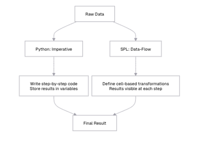
The first and most fundamental difference between Python and SPL are their programming paradigms. Python follows an imperative programming model, where you specify a sequence of operations to transform data. SPL, on the other hand, uses a dataflow programming model, where you define a series of steps that data flows through.
Python’s imperative programming model explained
In Python, you typically write code that explicitly states how to perform operations:
|
1 2 3 4 5 6 7 8 9 10 11 12 13 14 15 16 |
import pandas as pd # Load data sales_data = pd.read_csv("sales.csv") # Filter data high_value_sales = sales_data[sales_data['AMOUNT'] > 1000] # Group and aggregate region_totals = high_value_sales.groupby('REGION')['AMOUNT'].sum().reset_index() # Sort results sorted_totals = region_totals.sort_values('AMOUNT', ascending=False) # Display results print(sorted_totals) |
In this Python example, you create a series of variables that hold the intermediate results of your data transformations. The focus is on how to perform each step, and you need to track the flow of data through these variables. If you want to see intermediate results, you need to explicitly print them.
esProc SPL’s data-flow programming model explained
In SPL, you define a sequence of cells, each representing a step in your data processing workflow:
| A | |
| 1 | =file(“document/sales.csv”).import@ct() |
| 2 | =A1.select(AMOUNT>2000) |
| 3 | =A2.groups(REGION;sum(AMOUNT):TOTAL) |
| 4 | =A3.sort(TOTAL:-1) |
In SPL, each cell represents a transformation of the data, and the results flow naturally from one cell to the next. The focus is on what happens to the data at each step, rather than how to perform each operation. The results of each step are immediately visible in the IDE (integrated development environment) – unlike Python, where you must manually print intermediate results. This makes it easier to understand the data flow and verify that each step is working as expected in SPL.
Additionally, instead of variables, SPL uses cell references like A1, A2, and A3 to represent each step in the workflow, making the data flow more structured and transparent. This approach contrasts with Python, where the sequence of operations determines the flow implicitly.
By focusing on defining what needs to be done rather than detailing every step of how to do it, SPL can make data transformations more intuitive, especially when working with large datasets that require multiple processing steps.
Filtering and sorting: list comprehensions in Python vs. SPL’s A.select() and A.sort()
Python offers multiple ways to filter and sort data, including list comprehensions and Pandas methods. Let’s compare these with SPL’s approach.
Filtering data in Python/Pandas (option 1)
|
1 2 3 4 5 6 7 8 9 10 11 |
# Using boolean indexing laptops = sales_df[sales_df['PRODUCT'] == 'Laptop'] # Using query method high_value_laptops = sales_df.query("PRODUCT == 'Laptop' and AMOUNT > 1000") # Using list comprehension (with records) laptop_records = [row for row in sales_df.to_dict('records') if row['PRODUCT'] == 'Laptop'] print(f"Number of laptop sales: {len(laptops)}") print(f"Number of high-value laptop sales: {len(high_value_laptops)}") |
Filtering data in esProc SPL (option 1)
| A | ||
| 1 | =file(“document/sales.csv”).import@ct() | |
| 2 | =A1.select(PRODUCT==”Laptop”) | |
| 3 | =A2.len() 18 | |
| 4 | =A2.select(AMOUNT>1000) | Filtered for high-value laptops |
| 5 | =A4.len() 12 |
The output shows that there are 18 laptop sales in total (A3) and 12 high-value laptop sales (A5). This means that two-thirds of all laptop sales (12 out of 18) are high-value sales over $1,000. SPL’s `select` method provides a concise way to filter data based on conditions, and the results are immediately visible in the IDE.
Simple Talk is brought to you by Redgate Software
Filtering data in Python/Pandas (option 2)
|
1 2 3 4 5 6 7 8 9 |
# Filtering with multiple conditions complex_filter = sales_df[ (sales_df['REGION'].isin(['East', 'West'])) & (sales_df['AMOUNT'] > 1000) & ((sales_df['PRODUCT'] == 'Laptop') | (sales_df['PRODUCT'] == 'Server')) ] print(f"Complex filter results: {len(complex_filter)}") print(complex_filter.head(3)) |
Filtering data in esProc SPL (option 2)
| A | ||
| 1 | =file(“document/sales.csv”).import@ct() | |
| 2 | =A1.select((REGION==”East” || REGION==”West”) && AMOUNT>1000 && (PRODUCT==”Laptop” || PRODUCT==”Server”)) | |
| 3 | =A2.len() | 14 |
| 4 | =A2.to(3) | First 3 rows of filtered data |
The output of A3 shows that there are 14 rows matching the complex filter. These are high-value sales (over $1,000) of laptops or servers in the East or West regions. The output of A4 might look like:
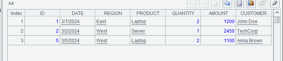
SPL’s syntax for complex conditions is more concise and readable than Pandas’ syntax, especially for nested conditions. The use of familiar operators like `==`, `&&`, and `||` makes the code more intuitive, particularly for those coming from programming languages like JavaScript or C#.
How do you sort data in Python/Pandas?
|
1 2 3 4 5 6 7 8 9 10 |
# Sort by a single column sorted_by_amount = sales_df.sort_values('AMOUNT', ascending=False) # Sort by multiple columns multi_sorted = sales_df.sort_values(['REGION', 'AMOUNT'], ascending=[True, False]) print("Sorted by AMOUNT (descending):") print(sorted_by_amount.head(3)) print("\nSorted by REGION (ascending) and AMOUNT (descending):") print(multi_sorted.head(3)) |
How do you sort data in esProc SPL?
| A | |
| 1 | =file(“document/sales.csv”).import@ct() |
| 2 | =A1.sort(AMOUNT:-1) |
| 3 | =A2.to(3) |
| 4 | =A1.sort(REGION,AMOUNT:-1) |
| 5 | =A4.to(3) |
The output of A3 might look like:
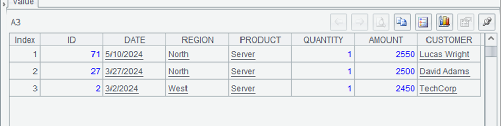
This shows the three highest-value sales in the dataset, sorted in descending order by amount. The highest sale is a server for $2,550, followed by another server sale for $2,500.
The output of A5 might look like:
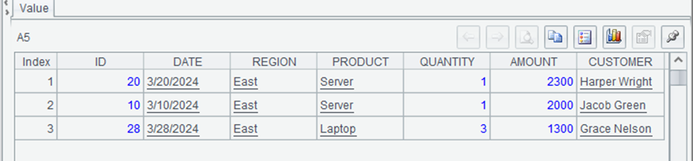
This shows the first three rows sorted by region (alphabetically) and then by amount (descending). All three rows are from the East region, with the highest-value sales listed first. SPL’s `sort` method provides a concise way to sort data by multiple columns in different directions.
When it comes to filtering and sorting, SPL offers a more concise and readable syntax compared to Pandas, particularly when dealing with complex conditions. It uses familiar logical operators like ==, &&, and ||, making expressions more intuitive, whereas Pandas relies on & and |, which require careful use of parentheses to avoid errors.
Sorting in SPL is also straightforward, as you can specify descending order with -1, while Pandas requires setting the ascending parameter to False. Both languages support chaining operations, but SPL’s cell-based execution allows you to inspect intermediate results more easily, making debugging and analysis more transparent.
Grouping and aggregation in Python vs esProc SPL – what are the differences?
Grouping and aggregation are common operations in data analysis, and both Python/Pandas and SPL provide powerful tools for these tasks. Let’s compare their approaches.
Grouping and aggregation in Python/Pandas (option 1)
|
1 2 3 4 5 6 7 8 9 10 11 12 13 14 15 |
# Group by REGION and sum AMOUNT region_totals = sales_df.groupby('REGION')['AMOUNT'].sum().reset_index() # Group by REGION and calculate multiple aggregates region_stats = sales_df.groupby('REGION').agg({ 'AMOUNT': ['sum', 'mean', 'count'] }).reset_index() # Rename columns for clarity region_stats.columns = ['REGION', 'TOTAL', 'AVERAGE', 'COUNT'] print("Region Totals:") print(region_totals) print("\nRegion Statistics:") print(region_stats) |
Grouping and aggregation in esProc SPL (option 1)
| A | |
| 1 | =file(“document/sales.csv”).import@ct() |
| 2 | =A1.groups(REGION;sum(AMOUNT):TOTAL) |
| 3 | =A1.groups(REGION; sum(AMOUNT):TOTAL, avg(AMOUNT):AVERAGE, count(AMOUNT):COUNT) Multiple aggregates |
The output of A2 might look like:
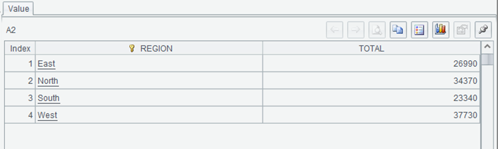
This shows the total sales amount for each region. The West region has the highest total sales at $37,730, followed by North at $34,370, East at $26,990, and South at $23,340.
The output of A3:
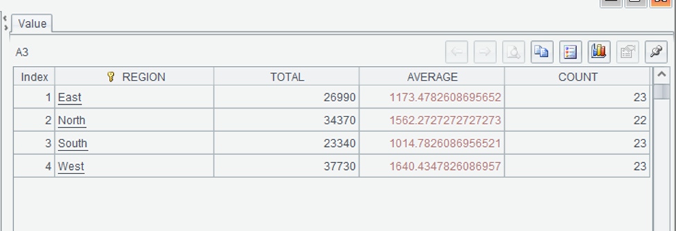
This provides a more comprehensive view of sales by region, including the total sales amount, average sale amount, and number of sales for each region. SPL’s `groups` method provides a concise way to calculate multiple aggregates in a single operation, with clear syntax for naming the resulting columns.
Grouping and aggregation in Python/Pandas (option 2)
|
1 2 3 4 5 6 7 8 9 10 11 12 13 |
# Group by multiple columns product_region = sales_df.groupby(['REGION', 'PRODUCT']).agg({ 'AMOUNT': ['sum', 'count'] }).reset_index() # Rename columns product_region.columns = ['REGION', 'PRODUCT', 'TOTAL', 'COUNT'] # Filter groups after aggregation high_volume = product_region[product_region['COUNT'] > 3] print("Product sales by region (high volume only):") print(high_volume) |
Grouping and aggregation in esProc SPL (option 2)
| A | |
| 1 | =file(“document/sales.csv”).import@ct() |
| 2 | =A1.groups(REGION, PRODUCT; sum(AMOUNT):TOTAL, count(AMOUNT):COUNT) Group by REGION and PRODUCT |
| 3 | =A2.select(COUNT>3) Filter for high-volume products |
The output of A3 might look like:
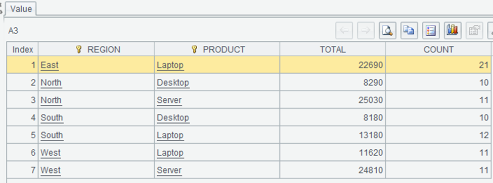
This shows the region-product combinations with more than 3 sales. Laptops are popular across all regions, with the highest total sales in the East region ($22,690). SPL’s approach to grouping and filtering is more concise and readable.
Subscribe to the Simple Talk newsletter
What is Python and esProc SPL’s equivalent to the SQL HAVING clause?
In SQL, the HAVING clause filters groups after aggregation. Let’s compare how Python and SPL handle this:
How does the HAVING clause work in Python/Pandas?
|
1 2 3 4 5 6 |
# Two-step process: group, then filter region_totals = sales_df.groupby('REGION')['AMOUNT'].sum().reset_index() high_total_regions = region_totals[region_totals['AMOUNT'] > 30000] print("Regions with total sales over $30,000:") print(high_total_regions) |
How does the HAVING clause work in esProc SPL?
| A | ||
| 1 | =file(“document/sales.csv”).import@ct() | |
| 2 | =A1.groups(REGION;sum(AMOUNT):TOTAL) Group by REGION and sum AMOUNT | |
| 3 | =A2.select(TOTAL>30000) | Filter for high-total regions |
SPL’s approach to post-aggregation filtering is similar to Pandas’. In esProc SPL, the groups method offers a clear and intuitive way to perform grouping and aggregation, separating grouping columns from aggregate expressions for better readability.
Unlike Pandas, where renaming aggregated columns often requires an additional step, SPL allows direct renaming within the groups method using the : syntax. Both languages support filtering results after aggregation, but SPL’s approach tends to be more concise.
Additionally, SPL simplifies calculating multiple aggregates in a single operation with a straightforward syntax for naming the resulting columns, reducing the need for extra processing steps.
Python’s datetime vs. esProc SPL’s built-in functions
Date and time manipulation is a common task in data analysis. Let’s compare how Python and SPL handle these operations.
How do basic date operations work in Python/Pandas?
|
1 2 3 4 5 6 7 8 9 10 11 12 13 14 15 |
import pandas as pd from datetime import datetime # Load CSV file and parse dates sales_df = pd.read_csv("sales.csv", parse_dates=['DATE']) # Define date range start_date = datetime(2023, 5, 1) end_date = datetime(2023, 5, 31) # Filter sales data within the date range may_sales = sales_df[(sales_df['DATE'] >= start_date) & (sales_df['DATE'] <= end_date)] # Display the number of sales in May 2023 print(f"Number of sales in May 2023: {len(may_sales)}") |
How do basic date operations work in esProc SPL?
| A | ||
| 1 | =file(“document/sales.csv”).import@ct() | |
| 2 | =A1.select(DATE>=date(“2023-05-01”) && DATE<=date(“2023-05-31”)) | Filter for May 2023 |
| 3 | =A2.len() | 28 |
The output of A3 shows that there are 28 sales in May 2023. SPL’s date functions make it easy to filter data by date range, with a syntax that’s similar to filtering by other types of values.
Extracting date components in Python vs esProc SPL
How does extracting date components work in Python/Pandas?
|
1 2 3 4 5 6 7 8 9 10 |
# Extract date components sales_df['YEAR'] = sales_df['DATE'].dt.year sales_df['MONTH'] = sales_df['DATE'].dt.month sales_df['DAY'] = sales_df['DATE'].dt.day # Group by month monthly_sales = sales_df.groupby('MONTH')['AMOUNT'].sum().reset_index() print("Monthly sales totals:") print(monthly_sales) |
How does extracting date components work in esProc SPL?
| A | ||
| 1 | =file(“document/sales.csv”).import@ct() | |
| 2 | =A1.groups(month(DATE):MONTH; sum(AMOUNT):TOTAL) |
The output of A2 will show the total sales for each month. SPL’s date functions make it easy to extract components from dates and use them for grouping and analysis.
What is the data arithmetic for extracting date components in Python/Pandas?
|
1 2 3 4 5 6 7 8 9 |
# Add 30 days to each date sales_df['FUTURE_DATE'] = sales_df['DATE'] + timedelta(days=30) # Calculate days between dates today = datetime.now().date() sales_df['DAYS_AGO'] = (today - sales_df['DATE'].dt.date).dt.days print("Dates with days ago:") print(sales_df[['DATE', 'DAYS_AGO']].head(3)) |
What is the data arithmetic for extracting date components in esProc SPL?
| A | ||
| 1 | =file(“document/sales.csv”).import@ct() | |
| 2 | =A1.derive(FUTURE_DATE:date(DATE).addDays(30)) | Add 30 days to each date |
| 3 | =A2.derive(interval(DATE,now()):DAYS_AGO) | Calculate days between dates |
| 4 | =A3.to(3).new(DATE,DAYS_AGO).peek(3) | First 3 rows |
The output of A4 shows the original date and the number of days between that date and today. SPL’s `interval@d` function calculates the number of days between two dates, similar to subtracting dates in Pandas.
When working with dates, both Pandas and esProc SPL offer a range of functions, but their approaches differ. In Pandas, you need to parse dates when loading data, while in SPL, the string dates will be automatically converted into date objects. SPL provides built-in functions like year(), month(), and day() that are directly called on date objects, whereas Pandas requires using the .dt accessor for similar operations.
Date arithmetic is also handled differently: SPL uses methods like elapse(), while Pandas relies on operators combined with timedelta. When calculating intervals between dates, SPL offers the interval@d function to return the number of days between two dates, which is similar to subtracting date objects in Pandas.
String manipulation in Python and esProc SPL: what are the differences, and how does it work in each?
String manipulation is another common task in data analysis. Let’s compare how Python and SPL handle these operations.
What are the basic string operations in Python/Pandas?
|
1 2 3 4 5 6 7 8 9 10 11 |
# Convert to uppercase sales_df['REGION_UPPER'] = sales_df['REGION'].str.upper() # Extract substring sales_df['REGION_FIRST_3'] = sales_df['REGION'].str[:3] # Concatenate strings sales_df['PRODUCT_REGION'] = sales_df['PRODUCT'] + " - " + sales_df['REGION'] print("String operations:") print(sales_df[['REGION', 'REGION_UPPER', 'REGION_FIRST_3', 'PRODUCT_REGION']].head(3)) |
What are the basic string operations in esProc SPL?
| A | ||
| 1 | =file(“document/sales.csv”).import@ct(REGION) | |
| 2 | =A1.derive(upper(REGION):REGION_UPPER,substr(REGION,1,3): REGION_FIRST_3,PRODUCT+” – “+REGION:PRODUCT_REGION) | String operations |
| 3 | =A2.to(3) | First three rows |
The output of A3 might look like:
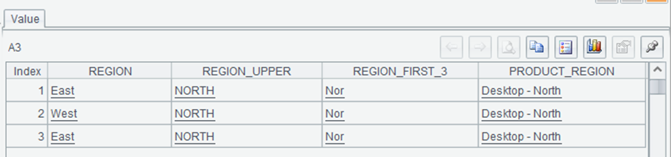
This shows the results of various string operations on the REGION column. The `upper` function converts the region to uppercase, the `substr` function extracts the first three characters, and the `+` operator concatenates the product and region with a separator. SPL’s string functions are similar to Python’s, but with a more integrated approach that allows you to perform multiple operations in a single `derive` call.
How to string search and replace in Python and esProc SPL
How do you string search and replace in Python/Pandas?
|
1 2 3 4 5 6 7 8 |
# Check if string contains substring sales_df['HAS_EAST'] = sales_df['REGION'].str.contains('East') # Replace substring sales_df['REGION_MODIFIED'] = sales_df['REGION'].str.replace('East', 'Eastern') print("String searching and replacing:") print(sales_df[['REGION', 'HAS_EAST', 'REGION_MODIFIED']].head(5)) |
How do you string search and replace in esProc SPL?
| A | ||
| 1 | =file(“document/sales.csv”).import@ct(REGION) | |
| 2 | =A1.derive(pos(REGION,”East”)>0: HAS_EAST, replace(REGION,”East”,”Eastern”):REGION_MODIFIED) | String searching and replacing |
| 3 | =A2.to(5) | First five rows |
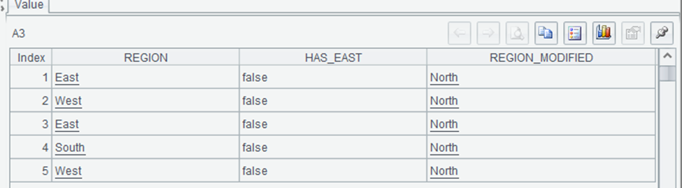
This shows the results of string searching and replacing operations. The `pos` function returns the position of a substring within a string, and we use `pos(REGION,”East”)>0` to check if the region contains “East”. The `replace` function replaces all occurrences of a substring with another string. SPL’s string functions provide similar capabilities to Python’s, but with a syntax that integrates well with other data operations.
How regular expressions work in Python and esProc SPL
How do regular expressions work in Python/Pandas?
|
1 2 3 4 5 6 7 8 9 10 11 |
import re # Extract digits from product names def extract_digits(text): match = re.search(r'\d+', str(text)) return match.group(0) if match else "" sales_df['PRODUCT_DIGITS'] = sales_df['PRODUCT'].apply(extract_digits) print("Regular expression extraction:") print(sales_df[['PRODUCT', 'PRODUCT_DIGITS']].head(5)) |
How do regular expressions work in esProc SPL?
| A | |
| 1 | =file(“document/sales.csv”).import@ct(PRODUCT) |
| 2 | =A1.derive(PRODUCT.regex(“[^\d]*(\d+)”):PRODUCT_DIGITS) |
| 3 | =A2.to(3) |
esProc SPL allows for efficient string manipulation and regular expression operations directly within its functional framework. In this example, we first append a version number to each product name and then extract the digits using a regex-based approach. Unlike Python’s Pandas, where string operations require the str accessor and method chaining, SPL applies transformations directly to data columns, making expressions more concise.
And, while Python offers greater flexibility in handling complex regex patterns, SPL integrates string processing directly into data manipulation steps, reducing the need for additional function calls like `apply()’.
Summary and next steps
In this article, we’ve compared Python and esProc SPL across various aspects of data analysis, from basic operations to complex transformations. While both languages are good tools for data analysis, they approach the task from different perspectives.
As a Python developer, adding SPL to your toolkit doesn’t mean abandoning Python. Instead, it gives you another perspective on data analysis and another tool for specific tasks where SPL’s approach might be more efficient or intuitive.
Click here for more in the “Moving from Python to esProc SPL” series.
FAQs: Data analysis in Python and esProc SPL
1. Why should a Python user consider esProc SPL for data analysis?
esProc SPL offers a different approach to data analysis that can be more intuitive for certain tasks. Its cell-based, data-flow programming model makes complex data transformations easier to understand and debug. The immediate visibility of results at each step helps you identify issues early and iterate quickly. While Python excels at general-purpose programming and has a vast ecosystem, esProc SPL can be more efficient for data transformation workflows, especially when working with tabular data.
2. Does esProc SPL have built-in functions like Pandas?
Yes, esProc SPL provides built-in filtering, sorting, grouping, and aggregation functions.
3. How does data grouping in esProc SPL compare to Python’s `groupby()`?
esProc SPL’s `groups()` function achieves grouping and aggregation in one step.
4. Is esProc SPL faster than Pandas for large datasets?
Performance depends on the specific operation and dataset size. esProc SPL is optimized for data processing operations and can be faster than Pandas for certain tasks, especially those involving complex transformations of tabular data. Also, its memory management is designed specifically for data processing, which can lead to better performance for large datasets. However, for large datasets that exceed memory capacity, both tools offer options for processing data in chunks or connecting to external databases.
This document contains proprietary information and is protected by copyright law.
Copyright © 2026 Red Gate Software Limited. All rights reserved


Load comments