A company I worked for had a well-defined need for versioned data. In a lot of databases and applications we didn’t do updates or deletes – we did inserts. That means we had to have mechanisms for storing the data in such a way that we could pull out the latest version, a particular version, or data as of a moment in time. We solved this problem by using a version table that maintains the order in which data was edited across the entire database, by object. Some tables will basically have a new row for each new version of the data. Some may only have one or two new rows out of a series of new versions. Other tables would have 10s or even 100s of rows of data for a version. To get the data out of these tables, you have to have a query that looks something like this, written to return the latest version:

You can write this query using MAX or ROW_NUMBER and you can use CROSS APPLY instead of joining. All of these different approaches will return the data appropriately. Depending on the query and the data, each one results in differences in performance. These differences in performance really make the task of establishing a nice clean “if it looks like this, do that” pattern very difficult for developers to follow. I decided to set up a wide swath of tests for these methods in order to establish as many of the parameters around which one works best, given a reasonably well defined set of circumstances.

Database & Data

I designed a small database to show versions of data. The initial design had a clustered index on each of the primary keys and you’ll note that many of the primary keys are compound so that their ordering reflects the ordering of the versions of the data.

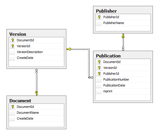
Figure 1

I used Red Gate’s SQL Data Generator to load the sample data. I tried to go somewhat heavy on the data so I created 100,000 Documents, each with 10 versions. There were 5,000 Publishers. All of this came together in 4,000,000 Publications. After the data loads, I defragmented all theindexes. All performance will be recorded in terms of reads and scans since duration is too dependent on the machine running the query. I will report execution times though, just to have another point of comparison.

Simple Tests to Start

The simplest test is to look at pulling the TOP (1), or MAX version, from the version table, not bothering with any kind of joins or sub-queries or other complications to the code. I’m going to run a series of queries, trying out different configurations and different situations. Each query run will include an actual execution plan, disk I/O and execution time. I’ll also run DBCC FREEPROCCACHE and FREESYSTEMCACHE (‘ALL’) prior to each query to try to get an apples-to-apples comparison. I’ll start with:

The first result generated a single scan with three reads in 5ms and this execution plan:

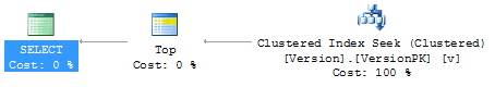
Figure 2

Next I’ll run a simple version of the MAX query using a sub-select.

This query provides a 5ms execution with one scan and three reads and the following, identical, execution plan:

Figure 3

Finally, the ROW_NUMBER version of the query:

Which resulted in an 46ms long query that had one scan and three reads, like the other two queries. It resulted in a slightly more interesting execution plan:

Figure 4

Clearly, from these examples the faster query is not really an issue. In fact, any of these processes will work well, although at 46ms, the ROW_NUMBER query was a bit slower. The execution plans for both TOP and MAX were identical with a Clustered Index Seek followed by a Top operation. While the ROW_NUMBER execution plan was different, the cost was still buried within the Clustered Index Seek and the query itself didn’t add anything in terms of scans or reads. So we’re done, right?

Not so fast. Now let’s try this with joins.

1 Join

Now we’ll perform the join operation from the Document table to the Version table. This will still only result in a single row result set. First, the TOP query:

The query ran in 37ms. This query had 2 scans against the Version table and 6 reads and only 2 reads against the Document table. The execution plan is just a little more complex than the previous ones:

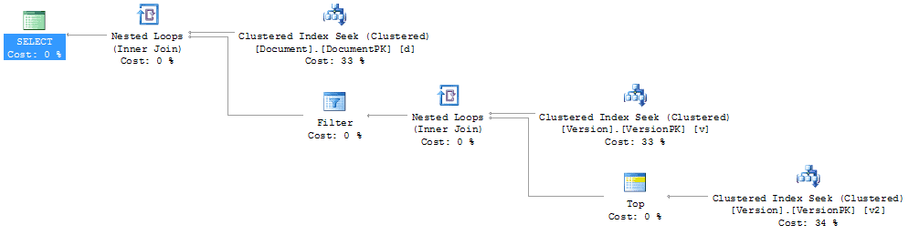
Figure 5

Now the MAX query:

This query ran in 32ms. It had 1 scan against the Version table and a combined 5 reads against both tables. The execution plan is as simple as the query itself:

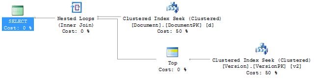
Figure 6

Explanations

In the last query, the optimizer chose to implement the MAX operation in the same way it did in the original simple example of MAX. But the TOP function forced the optimizer to join the data using a Nested Loop. This resulted in 2 scans of 6 reads each because the top query in the join returned all 10 rows for the Document ID provided. But what happens if we change the query just slightly. Instead of referencing the Version table for its DocumentId, I’ll reference the Document table like this:

Now when we run the query, there are one scan and six reads on the Version table with this execution plan.

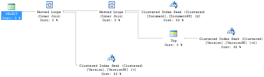
Figure 7

In this instance the TOP operator is still forcing a join on the system, but instead of looping through the Version records it’s doing a single read due to referring to the Document table directly. Now what happens if I change the query again? This time I’ll use the APPLY statement as part of the join:

This time the query has a single scan on Version and a total of five reads on both tables, and this familiar execution plan:

Figure 8

So the APPLY method was able to take the single row from the Document table and find that TOP (1) match from the Version table without resorting to joins and multiple scans.

and ROW_NUMBER

What happened to the ROW_NUMBER function? Here’s how that query has been rewritten.

This query resulted in the standard single scan with five reads and ran for 48ms, but had a radically different execution plan:

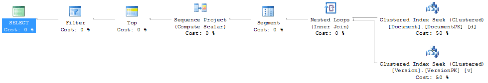
Figure 9

This query only accesses each table once, performing a clustered index seek operation. Also, like the others, the results of these seeks are joined through a Nested Loop operation. Next, instead of a TOP operator the data gets segmented by the Segment operator based on an internal expression, a value derived within the query, probably the ORDER BY statement. This is passed to the Sequence Project operator, which is adding a value; in this case, the ROW_NUMBER or RowNum column itself. And finally, the TOP and FILTER operators reduce the number of rows returned to one. While this appears to be more work for the query engine, it’s performing roughly on par with the other operations.

Full Data Set

Finally, let’s join all the data together. What we want is a list of publications, each demonstrating the max version that is less than a given maximum version. This is determining all the versions at a particular point in time. Here’s the new TOP, this time using APPLY right out of the gate because that proved earlier to result in a faster query:

The complete query ran in 53ms. Here are the scans and reads:

And this execution plan:

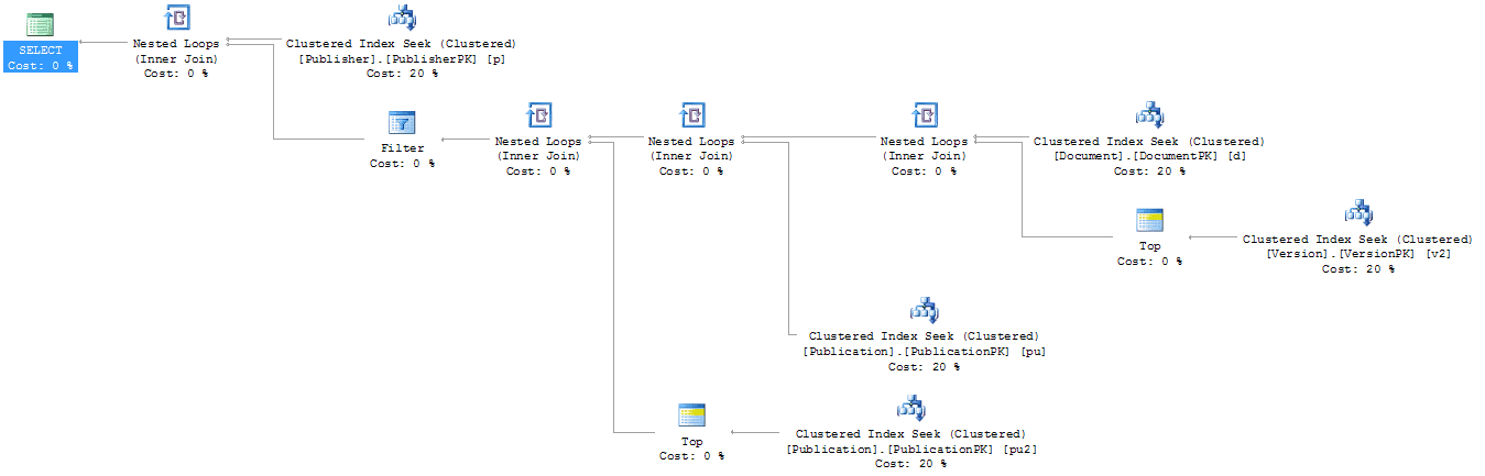
Figure 10

It’s a bit hard to read, but it’s a series of five Clustered Index Seek operations, each taking 20% of the total cost of the batch and joined together through Nested Loop joins. This is as clean and simple a plan as you can hope for.

Here is the MAX version of the FROM clause:

This query ran in 46ms. Its scans and reads break down as follows:

It resulted in a very similar execution plan:

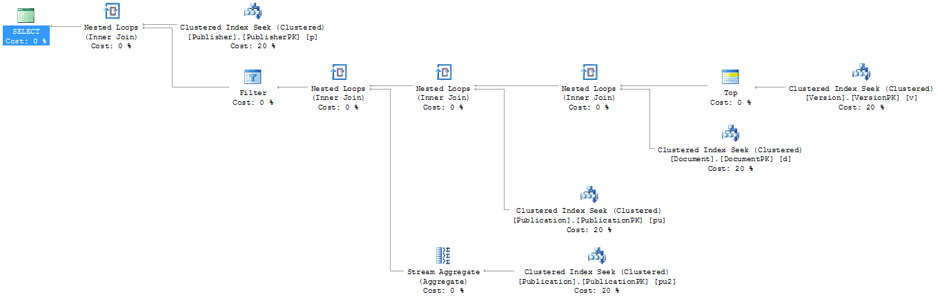
Figure 11

The execution plan consists of nothing except Clustered Index Seek and Nested Loop operators with a single TOP against the Version table. You would be hard pressed to come up with a better execution plan. The interesting thing is that the optimizer changed our MAX to a TOP as if we had re-supplied the TOP query. The only real difference is the order in which the tables are accessed, despite the fact that the queries submitted were identical. If the queries are run side-by-side, each takes exactly 50% of the cost of execution of the batch. There really isn’t a measurable difference.

And then the query itself changes for the ROW_NUMBER version (thanks to Matt Miller for helping with this one):

This query ran in 44ms and had an interesting set of scans and reads:

This query returned the exact same data with fewer scans and reads. In some ways it’s a bit more cumbersome than the other queries, but based on the scans and reads alone this is an attractive query. Even the execution plan, although slightly more complex, shows the increase in performance this approach could deliver.

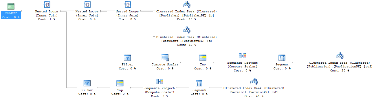
Figure 12

Instead of five Clustered Index Seeks, this has only four. There is some extra work involved in moving the data into the partitions in order to get the row number out of the function, but then the data is put together with Nested Loop joins; again, fewer than in the other plans.

Changing Results

What if we change the results, though? Let’s take the same query written above and simply return more data from one part. In this case, we’ll remove the PublisherId from the where clause. Now when we run the queries at the same time, the estimated cost for the TOP is only taking 49% while the estimated cost of the MAX is 50%. The difference? It’s in the Stream Aggregate in the execution plan. Part of the execution plan for the MAX uses TOP, just like the TOP query, but part of it uses an actual Aggregate operator. When the data set is larger, this operation suddenly costs more. But, interestingly enough, the execution times for the data I’m retrieving and the number of scans and reads are the same. Adding in the Row_Number query to run with other side by side was also interesting. In terms of execution plan cost, it was rated as the most costly plan. But look at these reads and scans:

The difference in scans on the Publication table, despite the fact that identical data was returned, is pretty telling for long term scalability. But that only went from selecting one row to selecting 10. The execution plans didn’t change and the differences were measured in very small amounts. Now instead of selecting by Document, I’ll change the query so that it selects by Publisher. Now the queries will have to process more data and return 100 rows. Everything changes.

The TOP query ran for 274ms with the following I/O

The elapsed time on the ROW_NUMBER ran up to 13 seconds. This is all from the change to using the PublisherId. Since it’s not part of the leading edge of the only index on the table – the PK – we’re forced to do a scan:

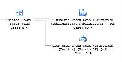
Figure 13

This is severe enough that it justifies adding another index to the table. If we simply add an index to Publication ID the scans are reduced, but not eliminated, because we’re then forced into an ID lookup operation:

Instead, we can try including the columns necessary for output, Publication Number and Publication Date; the other columns are included since they’re part of the primary key. This then arrives at the following set of scans and reads:

And this new execution plan:

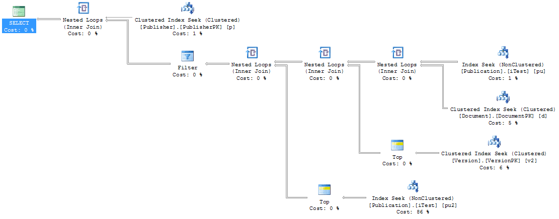
Figure 14

This then presents other problems because the Document table isn’t being filtered, resulting in more rows being processed. Rather than rewrite the queries entirely to support this new mechanism, we’ll assume this is the plan we’re going for and test the other approaches to the query against the new indexes. After clearing the procedure and system cache, the MAX query produced a different set of scans and reads:

The scans against Document and the number of reads against Version were less and the execution plan, a sub-set show here, was changed considerably:

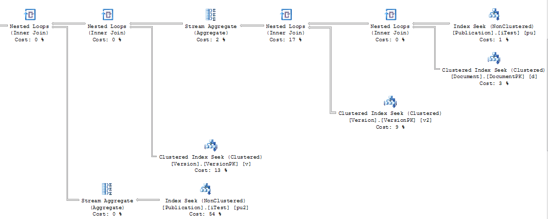
Figure 15

Instead of a scan against the Document table, this execution plan was able to take advantage of the filtering provided through the Version and Publication table prior to joining to the Document table. While this is interesting in overall performance terms, the differences in terms of which process, TOP or MAX, works better is not answered here. The MAX still results in a Stream Aggregate operation, which we already know is generally more costly than the Top operations.

The most dramatic change came in the ROW_NUMBER function. Execution time was 12 seconds. The test was re-run several times to validate that number and to ensure it wasn’t because of some other process interfering. Limiting based on PublicationId resulted in a pretty large increase in scans and reads, as well as the creation of a work tables:

The full execution plan is here:

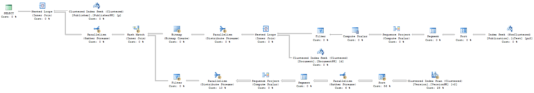
Figure 16

I’ve blown up a section of it for discussion here:

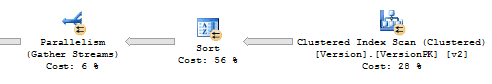
Figure 17

This shows that the Sort, which previously acted so quickly on smaller sets of data, is now consuming 56% of the estimated cost since the query can’t filter down on this data in the same fashion as before. Further, the total cost of the query is estimated at 277.188, far exceeding the cost threshold for parallelism that I have set on my machine of 50. The number of reads against the Version table makes this almost unworkable. The interesting point, though, is that the reads and scans against the other tables, especially the Publication table, are very low, lower than the other methods. With some rewriting it might be possible to get the performance on this back on par with the other processes.

Conclusion

When it comes to MAX or TOP, a well structured query running against good indexes should work well with either solution. This is largely because, more often than not, this type of query is interpreted in the same way by the optimizer whether you supplied a TOP or a MAX operator. It frequently substitutes TOP for the MAX operator. When this substitution is not made, the MAX value requires aggregation rather than simple ordering of the data and this aggregation can be more costly. TOP is probably the better solution in most instances when comparing MAX and TOP.

ROW_NUMBER clearly shows some strong advantages, reducing the number of operations, scans and reads. This works best on small sets of data. When the data sets are larger the processing time goes up quite a ways. So, to answer the questions, if you know the data set is going to be small, use ROW_NUMBER, but if the data set is going to be large or you’re not sure how large it’s going to be, use TOP. Having made this bold statement, please allow me to shade the answer with the following: test your code to be sure.