
SQL Server Data Warehouse Cribsheet
For things you need to know rather than the things you want to know
Contents
Introduction
One of the primary components in a SQL Server business intelligence (BI) solution is the data warehouse. Indeed, the data warehouse is, in a sense, the glue that holds the system together. The warehouse acts as a central repository for heterogeneous data that is to be used for purposes of analysis and reporting.
Because of the essential role that the data warehouse plays in a BI solution, it’s important to understand the fundamental concepts related to data warehousing if you’re working with such a solution, even if you’re not directly responsible for the data warehouse itself. To this end, the article provides a basic overview of what a data warehouse is and how it fits into a relational database management system (RDBMS) such as SQL Server. The article then describes database modelling concepts and the components that make up the model, and concludes with an overview of how the warehouse is integrated with other components in the SQL Server suite of BI tools.
- Note:
- The purpose of this article is to provide an overview of data warehouse concepts. It is not meant as a recommendation for any specific design. In addition, the article assumes that you have a basic understanding of relational database concepts such as normalization and referential integrity. In addition, the examples used in here tend to be specific to SQL Server 2005 and 2008, although the underlying principles can apply to any RDBMS.
The Data Warehouse
A data warehouse consolidates, standardizes, and organizes data in order to support business decisions that are made through analysis and reporting. The data might originate in RDBMSs such as SQL Server or Oracle, Excel spreadsheets, CSV files, directory services stores such as Active Directory, or other types of data stores, as is often the case in large enterprise networks. Figure 1 illustrates how heterogeneous data is consolidated into a data warehouse.
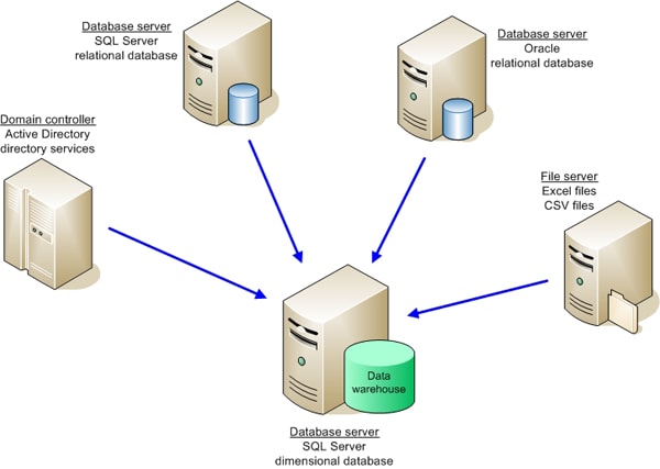
Figure 1: Using a Data Warehouse to Consolidate Heterogeneous Data
The data warehouse must be able to store data from a variety of data sources in a way that lets tools such as SQL Server Analysis Services (SSAS) and SQL Server Reporting Services (SSRS) efficiently access the data. These tools are, in effect, indifferent to the original data sources and are concerned only with the reliability and viability of the data in the warehouse.
A data warehouse is sometimes considered to be a place for archiving data; however, that is not its purpose. Although historical data is stored in a data warehouse, only the historical range necessary to support analysis and reporting is retained there. For example, if a business rule specifies that the warehouse must maintain two years worth of historical data, older data is offloaded to another system for archiving or is deleted, depending on the specified business requirements.
Data Warehouse vs. Data Mart
A data warehouse is different from a data mart, although the terms are sometimes used interchangeable. In addition, there is some debate as to what exactly constitutes a data mart as compared to a data warehouse. However, it is generally accepted that a data warehouse is associated with enterprise-wide business processes and decisions (and consequently is usually a repository for enterprise-wide data), whereas the data mart tends to focus on a specific business segment of that enterprise. In some cases, a data mart might be considered a subset of the data warehouse, although this is by no means a universal interpretation or practice. For the purposes of this article, we’re concerned only with the enterprise-wide repository known as a data warehouse.
Relational Database vs. Dimensional Database
Because SQL Server, like Oracle and MySQL, is a RDBMS, any database stored within that system can be considered, by extension, a relational database. And that’s where things can get confusing.
The typical relational database supports online transaction processing (OLTP). For example, an OLTP database might support bank transactions or store sales. The transactions are immediate and the data is current, with regard to the most recent transaction. The database conforms to a relational model for efficient transaction processing and data integrity. The database design should, in theory, adhere to the strict rules of normalization which aim, among other things, to ensure that the data is treated as atomic units and there is minimal amount of redundant data.
A data warehouse, on the other hand, generally conforms to a dimensional model, which is more concerned with query efficiency than issues of normalization. Even though a data warehouse is, strictly speaking, a relational database (because it’s stored in a RDBMS), the tables and relationships between those tables are modelled very differently from the tables and relationships defined in the relational database. (The specifics of data warehouse modelling are discussed below.)
- Note:
- Because of the reasons described above, you might come across documentation that refers to a data warehouse as a relational database. However, for the purposes of this article, I refer to an OLTP database as a relational database and a data warehouse as a dimensional database.
Dimensional Database vs. Multidimensional Database
Another source of confusion at times is the distinction between a data warehouse and an SSAS database. The confusion results because some documentation refers to an SSAS database as a dimensional database. However, unlike the SQL Server database engine, which supports OLTP as well as data warehousing, Analysis Services supports online analytical processing (OLAP), which is designed to quickly process analytical queries. Data in an OLAP database is stored in multidimensional cubes of aggregated data, unlike the typical table/column model found in relational and dimensional databases.
- Note:
- I’ve also seen a data warehouse referred to as a staging database when used to support SSAS analysis. Perhaps from an SSAS perspective, this might make sense, especially if all data in the data warehouse is always rolled up into SSAS multidimensional cubes. In this sense, SSAS is seen as the primary database and the warehouse as only supporting that database. Personally, I think such a classification diminishes the essential role that the data warehouse plays in a BI solution, so I would tend to avoid this sort of reference.
OLAP technologies are usually built with dimensionally modelled data warehouses in mind, although products such as SSAS can access data directly from relational database. However, it is generally recommended to use a warehouse to support more efficient queries, properly cleanse the data, ensure data integrity and consistency, and support historical data. The data warehouse also acts as a checkpoint (not unlike a staging database!) for troubleshooting data extraction, transformation, and load (ETL) operations and for auditing the data.
The Data Model
A data warehouse should be structured to support efficient analysis and reporting. As a result, the tables and their relationships must be modelled so that queries to the database are both efficient and fast. For this reason, a dimensional model looks very different from a relational model.
There are basically two types of dimensional models: the star schema and snowflake schema. Often, a data warehouse model follows one schema or the other. However, both schemas are made up of the same two types of tables: facts and dimensions. Fact tables represent a core business process, such as retail sales or banking transactions. Dimension tables store related details about those processes, such as customer data or product data. (Each table type is described in greater detail later in the article.)
The Star Schema
The basic structure of a star schema is a fact table with foreign keys that reference a set of dimensions. Figure 2 illustrates how this structure might look for an organization’s sales process.
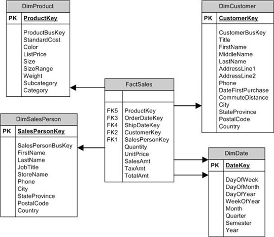
Figure 2: Using a Star Schema for Sales Data
The fact table (FactSales) pulls together all information necessary to describe each sale. Some of this data is accessed through foreign key columns that reference dimensions. Other data comes from columns within the table itself, such as Quantity and UnitPrice. These columns, referred to as measures, are normally numeric values that, along with the data in the referenced dimensions, provide a complete picture of each sale.
The dimensions, then, provide details about the functional groups that support each sale. For example, the DimProduct dimension includes specific details about each product, such as color and weight. Notice, however, that the dimension also includes the Category and Subcategory columns, which represent the hierarchical nature of the data. (Each category contains a set of subcategories, and each subcategory contains a set of products.) In essence, the dimension in the star schema denormalizes-or flattens out-the data. This means that most dimensions will likely include a fair amount of redundant data, thus violating the rules of normalization. However, this structure provides for more efficient querying because joins tend to be much simpler than those in queries accessing comparable data in a relational database.
Dimensions can also be used by other fact tables. For example, you might have a fact that references the DimProduct and DimDate dimensions as well as references other dimensions specific to that fact. The key is to be sure that the dimension is set up to support both facts so that data is presented consistently through each one.
The Snowflake Schema
You can think of the snowflake schema as an extension of the star schema. The difference is that, in the snowflake schema, dimensional hierarchies are extended (normalized) through multiple tables to avoid some of the redundancy found in a star schema. Figure 3 shows a snowflake schema that stores the same data as the star schema in Figure 2.
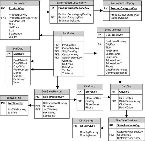
Figure 3: Using a Snowflake Schema for Sales Data
Notice that the dimensional hierarchies are now extended into multiple tables. For example, the DimProduct dimension references the DimProductSubcategory dimension, and the DimProductSubcategory dimension references the DimProductCategory dimension. However, the fact table still remains the hub of the schema, with the same foreign key references and measures.
The Star Schema vs. the Snowflake Schema
There is much debate over which schema model is better. Some suggest-in fact, insist-that the star schema with its denormalized structure should always be used because of its support for simpler and better performing queries. However, such a schema makes updating the data a more complex process. The snowflake schema, on the other hand, is easier to update, but queries are more complex. At the same time, there’s the argument that SSAS queries actually perform better against a snowflake schema than a star schema. And the debate goes on.
In many cases, data modellers choose to do a hybrid of both, normalizing those dimensions that support the user the best. The AdventureWorksDW and AdventureWorksDW2008 sample data warehouses take this approach. For example, in the AdventureWorksDW2008 database, the hierarchy associated with the DimProduct dimension is extended in a way consistent with a snowflake schema, but the DimDate dimension is consistent with the star schema, with its denormalized structure. The important point to keep in mind is that the business requirements must drive the data model-with query performance a prime consideration.
The Fact Table
At the core of the dimensional data model is the fact table. As shown in figures 2 and 3, the fact table acts as the central access point to all data related to a specific business process-in this case, sales. The table is made up of columns that reference dimensions (the foreign keys) and columns that are measures. A fact table supports several types of measures:
- Additive: A type of measure in which meaningful information can be extracted by aggregating the data. In the preceding examples, the SalesAmt column is additive because those figures can be aggregated based on a specified date range, product, salesperson, or customer. For example, you can determine the total sales amount for each customer in the past year.
- Nonadditive: A type of measure that does not expose meaningful information through aggregation. In the above examples, the UnitPrice column might be considered nonadditive. For example, totaling the column based on a salesperson’s sales in the past year does not produce meaningful data. Ultimately, a measure is considered nonadditive if it cannot be aggregated along any dimensions. (If a measure is additive along some dimensions and not others, it is sometimes referred to as semiadditive.)
- Calculated: A type of measure in which the value is derived by performing a function on one or more measures. For example, the TotalAmt column is calculated by adding the SalesAmt and TaxAmt values. (These types of columns are sometimes referred to as computed columns.)
If you refer back to figure 2 or 3, you’ll see that no primary key has been defined on the fact table. I have seen various recommendations on how to handle the primary key. One recommendation is to not include a primary key, as I’ve done here. Another recommendation is to create a composite primary key based on the foreign-key columns. A third recommendation is to add an IDENTITY column configured with the INT data type. Finally, another approach is to add columns from the original data source that can act as the primary key. For example, the source data might include an OrderID column. (This is the approach taken by the AdventureWorksDW2008 data warehouse.)
As stated above, the goal of any data warehouse design should be to facilitate efficient and fast queries (while still ensuring data integrity). However, other considerations should include whether it will be necessary to partition the fact table, how much overhead additional indexing (by adding a primary key) will be generated, and whether the indexing actually improves the querying process. As with other database design considerations, it might come down to testing various scenarios to see where you receive your greatest benefits and what causes the greatest liabilities.
The Dimension
A dimension is a set of related data that supports the business processes represented by one or more fact tables. For example, the DimCustomer table in the examples shown in figures 2 and 3 contains only customer-related information, such as name, address, and phone number, along with relevant key columns.
The Surrogate Key
Notice that the DimCustomer dimension includes the CustomerKey column and the CustomerBusKey column. Let’s start with CustomerKey.
The CustomerKey column is the dimension’s primary key. In most cases, the key will be configured as an IDENTITY column with the INT data type. In a data warehouse, the primary key is usually a surrogate key. This means that the key is generated specifically within the context of the data warehouse, independent of the primary key used in the source systems.
You should use a surrogate for a number of reasons. Two important ones are that the key provides the mechanism necessary for updating certain types of dimension attributes over time and it removes the dependencies on keys originating in different data sources. For example, if you retrieve customer data from two SQL Server databases, a single customer might be associated with multiple IDs or the same ID might be assigned to multiple customers.
That doesn’t mean that the original primary key is discarded. The original key is carried into the dimension and maintained along with the surrogate key. The original key, usually referred to as the business key, lets you map the source data to the dimension. For example, the CustomerBusKey column in the DimCustomer dimension contains the original customer ID, and the CustomerKey column contains the new ID (which is the surrogate key and primary key).
The Date Dimension
A date dimension (such as the DimDate dimension in the examples) is treated a little differently from other types of dimension. This type of table usually contains one row for each day for whatever period of time is necessary to support an application. Because a date dimension is used, dates are not tracked within the fact table (except through the foreign key), but instead in the referenced date dimension. This way, not only is the day, month, and year stored, but also such data as the week of the year, quarter, and semester. As a result, this type of information does not have to be calculated within the queries. This is important because date ranges usually play an important role in both analysis and reporting.
- Note:
- The DimDate dimension in the examples uses only the numerical equivalents to represent day values such as day of week and month. However, you can create a data dimension that also includes the spelled-out name, such as Wednesday and August.
A fact table can reference a date dimension multiple times. For instance, the OrderDateKey and ShipDayKey columns both reference the DateKey column in DimDate. If you also want to track the time of day, your warehouse should include a time dimension that stores the specific time increments, such as hour and minute. Again, a time dimension can be referenced by multiple facts or can be referenced multiple times within the same fact.
Unlike other types of dimensions whose primary key is an integer, a date dimension uses a primary key that represents the date. For example, the primary key for the October 20, 2008 row is 20081020. A time dimension follows the same logic. If the dimension stores hours, minutes, and seconds, each row would represent a second in the day. As a result, the primary key for a time such as 10:30:27 in the morning would be 103027.
The Slowly Changing Dimension
Dimension tables are often classified as slowly changing dimensions (SCDs), that is, the stored data changes relatively slowly, compared to fact tables. For instance, in the previous examples, the FactSales table will receive far more updates than the DimProduct or DimSalesPerson dimensions. Such dimensions normally change very slowly.
The way in which you identify a SCD affects how the dimension is updated during the ETL process. There are three types of slowly changing dimensions:
- Type 1: Rows to be updated are overwritten, thus erasing the rows history. For example, if the size of a product changes (which is represented as one row in the DimProduct dimension), the original size is overwritten with the new size, and there is no historical record of the original size.
- Type 2: Rows to be updated are added as new records to the dimension. The new record is flagged as current, and the original record is flagged as not current. For example, if the product’s color changes, there will be two rows in the dimension, one with the original color and one with the new color. The row with the new color is flagged as the current row, and the original row is flagged as not current.
- Type 3: Updated data is added as new columns to the dimension. In this case, if the product color changes, a new column is added so that the old and new colors are stored in a single row. In some designs, if the color changes more than once, only the current and original values are stored.
The built-in mechanisms in SQL Server Integration Services (SSIS) implement only Type 1 and Type 2 SCDs. Although you can build an ETL solution to work with Type 3 SCDs, Type 2 SCDs are generally considered more efficient, easier to work with, and provide the best capacity for storing historical data.
When working with SCDs in SSIS, you can use the Slowly Changing Dimension transformation to implement the SCD transformation workflow. However, SSIS does not identify SCDs at the dimension level, but rather at the attribute (column) level. Figure 4 shows the Slowly Changing Dimension Columns screen of the Slowly Changing Dimension wizard.
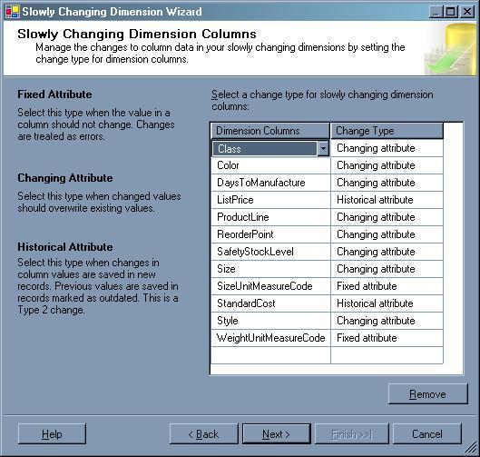
Figure 4: Specifying the Slowly Changing Dimension Columns in SSIS
For each column you can choose whether that column is a Changing Attribute (Type 1) or a Historical Attribute (Type 2). The wizard also offers a third option-Fixed Attribute, in which case, the value of the column can never change.
There is one other consideration when working with SCDs. If a dimension supports Type 2 SCDs, you need some way to mark each row to show whether it is the current row (the most recent updated row) and the historical range of when each row was current. The most effective way to do this is to add the following three columns to any dimension that supports SCD attributes:
- Start date: The date/time when the row was inserted into the dimension.
- End date: The date/time when the row became no longer current and a new row was inserted to replace this row. If the row is the most current row, this column value is set to null or assigned a maximum date that is out of the present-day range, such as December 31, 9999.
- Current flag: A Boolean or other indicator that marks which row within a given set of associated rows is the current row.
Some systems implement only the start date and end date columns, without a flag, and then use the end date to calculate which row is the current row. In fact, the Slowly Changing Dimension transformation supports using only the dates or using only a flag. However, implementing all three columns is generally considered to be the most effective strategy when working with SCDs. One approach you can take when using the Slowing Changing Transformation wizard is to select the status flag as the indicator and then modify the data flow to incorporate the start and end date updates.
The Data
Although the data warehouse is an essential component in an enterprise-wide BI system, there are indeed other important components. Figure 5 provides an overview of how the SQL Server suite of tools might be implemented in a BI system.
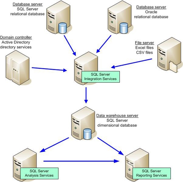
Figure 5: The SQL Server BI Suite
As you can see, SSIS provides the means to retrieve, transform, and load data from the various data sources. The data warehouse itself is indifferent to the source of the data. SSIS does all the work necessary to ensure that the data conforms to the structure of the warehouse, so it is critical that the warehouse is designed to ensure that the reporting and analysis needs are being met. To this end, it is also essential to ensure that the SSIS ETL operation thoroughly cleanses the data and guarantees its consistency and validity. Together SSIS and the data warehouse form the foundation on which all other BI operations are built.
After the data is loaded into the warehouse, it can then be processed into the SSAS cubes. Note that SSIS, in addition to loading the data warehouse, can also be used to process the cubes as part of the ETL operation.
In addition to supporting multidimensional analysis, SSAS supports data mining in order to identify patterns and trends in the data. SSAS includes a set of predefined data-mining algorithms that help data analyzers perform such tasks as forecasting sales or targeting mailings toward specific customers.
Another component in the SQL Server BI suite is SSRS. You can use SSRS to generate reports based on the data in either the data warehouse or in the SSAS database. (You can also use SSRS to access the data sources directly, but this approach is generally not recommended for an enterprise operation because you want to ensure that the data is cleansed and consistent before including it in reports.) Whether you generate SSRS reports based on warehouse data or SSAS data depends on your business needs. You might choose not to implement SSAS or SSRS, although it is only when these components are all used in orchestration that you realize the full power of the SQL Server BI suite.
Conclusion
Regardless of the components you choose to implement or the business rules you’re trying to address in your BI solution, you can see that the data warehouse plays a critical role in that solution. By storing heterogeneous and historical data in a manner that ensures data integrity and supports efficient access to that data, the data warehouse becomes the heart of any BI solution. As a result, the better you understand the fundamental concepts associated with the data warehouse, the more effectively you will understand and be able to work with all your BI operations.
This document contains proprietary information and is protected by copyright law.
Copyright © 2026 Red Gate Software Limited. All rights reserved


Load comments