Although relational division is defined in the relational algebra, it can be a challenging query for anyone, however experienced they are with SQL. Although it is the most effective way of tackling many database tasks, it is difficult enough just to identify those particular business requirements that are best solved by relational division. We’ll be trying to help with this, and also provide some code patterns that can be used to deliver high-performance results.

Relational division is the method that is used, for example, to identify:

• Candidates for a job requirement having the skills that job requires (the primary example used in this article).
• Orders containing only a specific subset of items.
• Customers that have an operating area in two or more specific locations.
• Parts that are shared across many Bills of Material (BOMs).
• Users that have the same distinct set of licensed software, e.g., MS Office, Windows XP and MS Visual Studio, installed on their machines.

In this article, I’ll be suggesting that the performance of almost every solution to relational division can be improved by reducing the rows as much as possible before applying the final logic.

While doing the research for this article, I stumbled across Divided We Stand: The SQL of Relational Division by renowned SQL author Joe Celko as published on Simple Talk. We’ll draw heavily on his examples of relational division because he does an excellent job of explaining them. We will change our data structures to offer you an alternative picture, in the hopes that additional examples may help to make it all clearer.

Problem Scenario and Data Setup

Firstly, we’ll need to create some sample data that we can use for most of the problems we’ll be exploring in this article. If you would like to follow along without having to copy/paste the queries from this article, you can download the attached resource file: 01 CandidatesSkills Sample Queries.sql, which contains all the sample queries related to our first example.

Let’s suppose you are a recruiting company. In your database you might have, in addition to a list of candidates and a list of all the skills your many clients are interested in (e.g., SQL, SSIS, SSRS, etc.), a table you might call CandidatesSkills. This is a mapping table of candidates to the skills they possess.

We’ll use, as is customary, IDs for both candidates and skills; but we will omit the related tables for Candidates and Skills because they’re not relevant to our focus. In relational division, the CandidatesSkills table is called the dividend table. This table needs good indexing to make any of the proposed queries in our article perform well.

We’ll now further suppose that a client comes along with a job opening, and for that job opening he has a list of skills that he seeks. He is one of our more demanding clients, so he insists that any candidate we present must have all of his listed skills. Let’s put this into a helper table, which in terms of relational division, is the divisor table.

Let’s now compare our sample data (candidates with their skills) to our requirement and identify the cases of relational division.

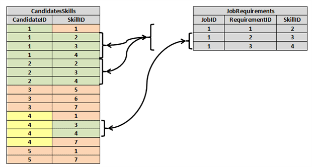
We have five candidates that seem to have relevant skills.

• Candidate 1 possesses all three required skills plus one additional
• Candidate 2 possesses only the three required skills
• Candidates 3 and 5 possess none of the required skills
• Candidate 4 possesses only two of the three required skills

Since Candidate 2 possesses only the required skills and no more, matching that candidate to the job posting is Relational Division with No Remainder (RDNR). Candidate 1 possesses the required skills plus one more, so this is known as Relational Division With Remainder (RDWR), the remainder being the one additional skill that is not required. One could argue that since Candidate 4 fulfills two of the three requirements, this could be a case of relational division as well; but we’ve excluded that case because our client demanded that all required skills are possessed in order to qualify a candidate.

Relational Division with Remainder (RDWR)

Joe Celko provided two solutions to this problem in the referenced article. He indicated that one of them performs better than the other, and I agree. That solution is as follows:

It is interesting to note that in the article’s discussion thread SQL MVP Peter Larsson, who may be better known for his posts under the monikers PESO or SWEPESO, came along and suggested that there’s a faster solution to the RDWR problem which he posted in his Thinking Outside the Box blog entry named Proper Relational Division with Sets. In fact, the solution that he suggested for this problem is versatile enough to solve either of the RDWR or RDNR problems (refer to the comment on the last line of code to see how).

Both of these solutions yield the following results based on our sample data, which by simply reviewing the graphic we provided earlier you’ll see is correct:

It is, of course, important to test out your solution on a large set of data once you are satisfied that it is correct. For this purpose, we have provided a script in the attached resources files (02 Create Large CandidatesSkills Tables.sql) that interested readers can use to create two large tables of CandidatesSkills to support testing the performance of these two solutions. The results you get from these may depend to a certain extent on the dispersion of the data points within your data.

Is this the final word? Later on in this article I’ll show a technique that can be applied in conjunction with either of these solutions that can improve the performance of both.

Relational Division with no Remainder (RDNR)

For the case of RDNR, Joe also provided a solution in his article. In PESO’s blog, he actually expanded that solution set to four, presumably based on correspondence with Joe. According to my testing, the fastest of those was this one. You can try to reproduce these results for yourself using 03 Test of RDNR Solutions at 1M Rows.sql.

When I looked at this, a slight improvement came to mind and testing confirmed that this variant is slightly faster.

Also in his blog, PESO provided a solution that represents a collaboration between him and SQL MVPAdam Machanic.

All three of these solutions produce the expected result from our sample data, which is:

Once again, we are not here today to compare how these solutions perform against each other. Instead we will now provide you a method whereby any of the solutions proposed so far (we’ll refer to these as the base queries) can be improved for huge row sets.

Improving Upon Relational Division with and without Remainder

Consider the query below, which we’ve built specifically to identify candidates that meet, some but not necessarily all, of the divisor criteria.

This produces the following results set:

This result set has some very interesting properties:

• It happens to contain only the CandidateIDs that would satisfy the RDWR and RDNR cases. However if we were looking for more job requirements (>3) then it would also contain additional rows that would need to be further checked to reduce the set down to just the target divisor.
• It contains all of the rows associated with the identified candidates.
• It is very fast with the indexes we created; producing exactly four index seeks in the query plan. Three of those seeks use the non-clustered INDEX on the table.

It does have a flaw however: If we happen to have less than 3 job requirements it won’t work. Let’s fix that and place this interesting new code into a Common Table Expression (CTE).

This will work even if there are less than three job requirements but at least one, and it still does the same four index seeks. The reason it works is that it “short circuits” the EXISTS check when one of the first three elements is NULL (meaning it doesn’t exist). Even more interesting is that, since all it does is produce a subset of the rows we need to examine, we can combine it with any of the five solutions presented previously for RDNR and RDWR, simply by replacing references to the CandidatesSkills table with a reference to the CTE instead! For example, if we combine it with the PESO+Adam Machanic collaboration for RDNR, we get this:

This can be confirmed to produce the correct result set for our sample data. We call this the Row Reduction Approach to Relational Division.

In order to truly see the impact this has on performance of the base queries, we really need to ramp up the amount of test data in our harness. This has already been done for you by creating a table (CandidateSkills2) that has approximately 10 million rows in it. We can apply each of the five queries discussed so far with the Row Reduction Approach and graph this using each base query as the basis, meaning that we’ll show the amount of elapsed time used by the Row Reduction Approach as a percentage of the base query. You may reproduce these results by running 04 With and Without Row Reduction on 10M Rows.sql.

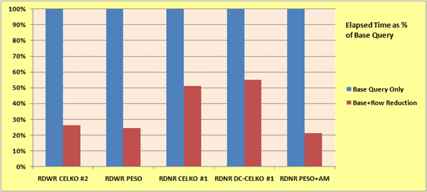
From these results it is clear that the Row Reduction Approach is beneficial in each case, reducing the elapsed time necessary to about 20-55% of that of the base query.

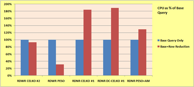
CPU usage is a bit more variable. For the RDWR problem it is generally less while for the RDNR problem generally more (and sometimes nearly twice as much). This may be a valid trade-off for the improvements in elapsed time.

Note once again that we have avoided comparing the raw speed of these five solutions against each other because that may depend on either the dispersal of the data in the dividend table and/or the number of elements to match against in the divisor table. In our case, each row reduction was applied three times. We experimented with more row reductions (up to seven in fact) and found in general that there will be a point of diminishing returns, after which more row reductions unfavorably impacts the elapsed time. The sweet spot with 10M rows of data seems to be around three or four row reductions. It may be a bit higher if you have hundreds of millions or billions of rows in your dividend table.

The bottom line here is that if you do relational division and have a favorite solution for it, using the row reductions technique (for large dividend tables) is very likely to provide you a faster performing solution.

Relational Division with Multiple Divisors

In our problems so far, we’ve been dealing with only a single, target subset of data (the divisor table) where we wish to identify the places where that data exists in our master table (the dividend table). You may be wondering why we included the column JobID in our divisor table; so now you get to find out.

Suppose we actually have two distinct job requirements. We can add the second job requirement to our divisor table like this:

Now we have the following data in our divisor table.

As before, depending on whether we want an exact division (RDNR) we’d get for JobID=1 the CandidateID of 2 or for division with remainder (RDWR) for JobID=1 we’d get CandidateIDs 1 and 2. But now we also want to return matches for JobID=2, which are 5 for RDNR and 4/5 for RDWR. In PESO’s blog, he enigmatically suggested that either of the queries he suggested could be modified to handle the case of multiple divisors, so let try to see if we can do that. We’ll choose the one that can be applied to either case.

It is quite easy to demonstrate (for the case shown) that this query returns:

It returns the following if MIN(cnt) >= 1.

The other queries we’ve discussed can be similarly modified to handle the case of multiple divisors.

The question before us though, is whether our Row Reduction Approach is also applicable. The answer is of course yes, albeit there is a limitation. In order to apply the Row Reduction Approach, we can only do it to the intersection of the job requirements. To make this work, we must modify the query that calculates the three variables we’ll use to do the row reduction to something that looks like this (assigning the intersection of the job requirements to our three variables).

We have modified the Row Reduction Approach (below) to handle the case where @XID1 can possibly be NULL. You may verify for yourself that the results are the same as before.

Clearly this limitation becomes more restrictive when you have more divisors; because the more you have, the less likely there will be an intersection that is anything but an empty set. However we’ve shown that it can be done. If there is then an overlap, it should still help to improve the performance of the query when you have a large dividend table.

Todd’s Division

Joe Celko also proposed another relational division problem he called Todd’s Division (because he attributed it to Stephen Todd). Once again, we will re-frame the problem to offer additional insight into the types of business problems that can be addressed.

We’ll start with a ProjectTasks table, which contains multiple projects and the tasks that are required for each. Note that a particular task may overlap various projects.

We also have a ResourceTasks table, which maps resources to tasks. Once again, a task may be assigned to multiple resources.

Our desired results set is a list of projects and the resources that are assigned to them based on which project that resources’ tasks are assigned to.

Joe Celko suggested that either of the following queries will return the desired results, and further suggested that the second one may be just a little faster in some cases (confirmed by me).

Both of these queries have two structures that, for performance reasons, I usually try to avoid where possible: a CROSS JOIN (disguised by the non-ANSI standard syntax that uses the comma between two tables) and DISTINCT. Cartesian products (from the CROSS JOIN) generate lots of unnecessary rows and DISTINCT can cause an expensive sort to occur. So let’s see if we can propose something just a little faster.

I’ve actually proposed two solutions because depending on the number of rows in your test harness, one or the other may be slightly faster. If you run 05 Test Harness for Todds Division.sql exactly as it is provided, you should see timing results similar to those shown below.

	Time (ms)
Query	Elapsed	CPU
Celko 1	14,109	37,209
Celko 2	14,251	37,144
Dwain.C 1	398	1,014
Dwain.C 2	392	1,186

If you follow the instructions within the test harness to increase the row counts,commenting out Joe Celko’s queries if you don’t want to wait for them to finish, you may find that at higher row counts my second solution is slightly faster (elapsed time) than my first. Both of these solutions represent a row reduction approach of a sort, because they use the INNER JOIN to reduce the rows that would otherwise be generated by the Cartesian product resulting from the CROSS JOIN.

This particular problem is immune from improvement by the Row Reduction Approach proposed for RDNR and RDWR, because of the number of entries in the divisor table. There would never be sufficient overlap to help reduce the execution time.

Romley’s Division

I have to give Joe Celko some credit here – for being a master of understatement. Romley’s Division (so named after Richard Romley of Salomon Smith Barney) is most certainly a quite complicated problem. Once again we’ll attempt to describe the problem but we’ll create an alternate scenario to help clarify when such a relational division might come into play.

Suppose we have a factory that has machines and assembly Lines. Each assembly line can support more than one process at a time: Each machine is uniquely associated with a single process, and can support only a single product at a time. We wish to determine for assembly lines and products, whether all, none or some of the processes are supported.

Let’s set up some sample data first and then we’ll look at possible solutions. First, the assembly lines and associated processes:

For the machines and their associated products/processes, we’ll start with this:

Joe Celko proposed the following query to solve Romley’s Division:

This produces the following results set:

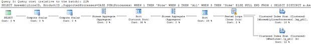
If you look at the query’s execution plan, you’ll find that this method uses just two clustered index scans. My initial feeling when I saw that suggested it was going to be pretty hard to beat.

I’m not ashamed to admit that just solving this bad boy took me awhile, but of course my job is especially challenging because I’m ultimately trying to come up with a faster query. After some more stumbling around (I seem to do that a lot), I came up with the following solution, which certainly looks more complicated but does at least deliver the expected results set.

The cost of the query’s execution plan for this approach is higher and it also looks quite a bit more complex.

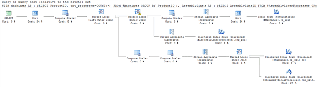I’ve often found from personal experience that query plan costs can be deceiving. The ultimate test is how it runs with a large test harness. So we built one that could be run for two cases.

	Attributes				Approximate Rows
Case	Assembly Lines	Machines	Products	Processes	#AssemblyLinesProcesses	#Machines
1	100	1,000	100	100	950	1,000
2	1,000	10,000	100	100	9,500	10,000

You can run the test yourself by using 06 Test Harness for Romleys Division.sql. It is initially set up to run Case 1, but you can uncomment some code near the beginning to run Case 2. The result that I got when I ran these cases was:

	Time (ms) – CELKO		Time (ms) – Dwain.C
Case	Elapsed	CPU	Elapsed	CPU
1	1,143	4,415	413	421
2	106,395	407,942	42,063	42,027

Somewhat surprisingly, this means that overall the elapsed time of my query for Romley’s Division was about 40% that of the original query, while it used only 10% of the CPU. The improvement is due to two main factors:

• The CROSS JOIN is applied to the two pre-aggregates, thus significantly reducing the size of the resulting Cartesian product. This gave me exactly the rows I needed for the first two columns of the final result.
• Using the INNER JOIN within the OUTER APPLY is sort of a row reduction of its own, and that is further reduced by the WHERE clause that limited the rows to only those applicable from the CROSS JOIN.

While not a case of using the originally proposed Row Reduction Approach (again it doesn’t apply here for various reasons), it shows that with a little effort a very tricky query can be turned into a high performance one.

Conclusion

I first was struck by the possibilities of the Row Reduction Approach to Relational Division when SQL MVPItzik Ben-Gan proposed a challenge to Identify a Subsequence within a Sequence. In part one of his article (link at left) I proposed three solutions in the post-article discussion, culminating in the Row Reduction Approach. In the discussion section of part two of the article, PESO commented that this was a special case of relational division that he called Ordered Relational Division. Also in that section, the performance results of the method were posted against the best solution proposed by the article. It was just slightly later that I realized what I had proposed could be generally applied to other more generic cases of relational division, illustrating my point early on that sometimes relational division is difficult to associate with a specific business problem. We’ll let you take a look at those two excellent articles to see what the fastest solution was.

The Row Reduction approach seems to improve the performance of any relational division query (with and without remainder), particularly if you are faced with exceedingly large row sets. This approach could even be used when your relational division has multiple remainders, albeit with some limitations.

The suggested Row Reduction approach cannot be applied to either Todd’s or Romley’s special relational division cases; but the key to achieving high performance queries in those instances also involves the principle of reducing the rows as much as possible prior to applying the final logic to solve the case.

A summary of the resource files (SQL scripts) provided with this article within the zip file at the bottom of the article follows:

• 01 CandidatesSkills Sample Queries.sql – Contains the sample data discussed in this article for RDWR, RDNR, and the sample queries for those cases (one with the Rows Reduction Approach) and for relational division with multiple divisors (i.e., all of the examples that use the CandidatesSkills table).
• 02 Create Large CandidatesSkills Tables.sql -This sets up two tables, CandidatesSkills1 and CandidatesSkills2 containing 1M and 10M rows respectively.
• 03 Test of RDNR Solutions at 1M Rows.sql – This verifies the solutions for RDNR at 1M rows so I could pick the best Joe Celko had to offer.
• 04 With and Without Row Reduction on 10M Rows.sql -This runs the five solutions we compared at 10M rows (refer to the two histograms provided).
• 05 Test Harness for Todds Division.sql – This contains a large test harness for all of the Todd’s Division queries. You can manually uncomment/comment some of the lines if you want to run as the sample queries in this section.
• 06 Test Harness for Romleys Division.sql – This contains a large test harness (Case 1) for all of the Romley’s Division queries. You can manually uncomment/comment some of the lines if you want to run as the sample queries in this section.