In this article, I’ll be showing a few techniques in pivoting and un-pivoting data, and showing you how the use of the CUBE or ROLLUP operator can be more efficient way of generating reports.
Why use Aggregate Tables?
I’ve always found it puzzling that Data Warehousing systems want to re-aggregate data over, and over again, especially if the data is time-based.
Imagine you have to report on a simple ledger. Ledgers, like most accounting entities, are based on written entries in leather-bound books. You start at the beginning, and add entries over time, but nothing is ever erased. Once an accounting for a period of time is done and balanced, then it is closed. Why then do we recalculate our trading figures, or past commercial activity, when no legitimate retrospective modifications are possible or valid? It is therefore bewildering to find reporting packages continually aggregating totals for particular time-periods from the raw data every time a report is run. Obviously, there are times when it is necessary to do so, but even when it is, it is possible to prevent a complete trawl of possibly millions of rows of data.
Business reports should always go to aggregation tables for their information wherever possible. This is especially true on production systems where the amount of data gets serious. An aggregation table often looks wrong to a Database Theorist because it looks suspiciously un-normalized. This is missing the point.
Aggregation operators
I find The ROLLUP, CUBE, and GROUPING SETS operators, which are extensions of the GROUP BY clause, to be useful for simplifying aggregation. Queries that contain CUBE and ROLLUP perform some of the same calculations as you’ll find in OLAP applications. The CUBE operator generates a result set that can be used for a variety of cross tabulation reports. A ROLLUP operation can calculate the equivalent of an OLAP dimension or hierarchy. They might, at first glance, seem slightly pointless until you start doing reports on large quantities of data.
The ROLLUP operator is perfect for any reports on data that have column totals. It means that you save a UNION ALL and an explicit second pass over the data
A CUBE comes into its own if you have several reports to produce from one source of data. Once you have performed the initial aggregation, and you have chosen your GROUP BY elements well, then you never have to access the original data, in order to slice and dice the data. All sorts of reports can be generated from the result of the CUBE just so long as you have specified the grouping properly. The cube performs all the possible permutations of the aggregation and adds them to the result.
You can, of course, generate the same result set when you use UNION ALL to combine single grouping queries; but the advantages of performing the query aggregation once really kicks in once you have millions of rows in your raw data tables. Using ROLLUP, CUBE, and GROUPING SETS is more efficient, though the SQL Server optimizer currently translates a CUBE into several ROLLUPs which operate on a common sub-expression spool, so it is not as efficient as a single-pass through the data.
The GROUPING SETS operator was introduced in SQL Server 2008 in order to conform with Ansi SQL 2006. The old syntax, WITH ROLLUP and WITH CUBE, which were functions that were intended for Data Warehousing, are found in SQL Server, and Sybase only. The Oracle version works like Ansi SQL 2006. The GROUPING SETS operator can generate the same result set as that generated by using a simple GROUP BY, ROLLUP, or CUBE operator. However, you can use GROUPING SETS to refine your query in order to specify only the groupings that you actually want. You can even use GROUPING SETS with ROLLUP and CUBE, but you are liable to get duplicate groupings, and you will probably make your head spin
A Simple Example
In this article, I’d like to do a round trip from published data, to a normalized table, through to an aggregation table and out to some reports. For our example, We want to do an analysis from external data. Just to make this more interesting, we’ll choose the oil production figures (thousand barrels per day) for the past nine years. These are available from Energy Information Administration (Oct 2008) from https://www.eia.gov/petroleum/supply/weekly/. The only downside is that it is not a multi-million row table, the sort of size where the use of an aggregation table makes solid sense.
We pick up four excel files. They are pivot-table reports done in the format…
|
Algeria |
Angola |
Argentina |
Australia |
… |
|
|
|
|||||
|
1997 Average |
1,277 |
714 |
834 |
588 |
… |
|
1998 Average |
1,246 |
735 |
847 |
544 |
… |
|
1999 Average |
1,202 |
745 |
802 |
539 |
… |
|
2000 Average |
1,254 |
746 |
761 |
722 |
… |
|
2001 January |
1,337 |
746 |
791 |
708 |
… |
|
February |
1,305 |
749 |
792 |
687 |
… |
|
March |
1,305 |
731 |
788 |
699 |
… |
|
April |
1,289 |
739 |
799 |
659 |
… |
|
May |
1,305 |
733 |
809 |
627 |
… |
|
June |
1,326 |
728 |
802 |
669 |
… |
|
… |
… |
… |
… |
… |
Now, this is all right for a report, but it ain’t a normalized table that we can work with. It is in a spreadsheet, and that seems a long way from our remote SQL server. First, we paste the four reports together to make one table. Then, we give it a little bit of a haircut in Excel so that we just get the raw data. We fix the dates so that we can export them to a database. (we simply put the start date in the top cell and just copy->fill-> series and choose a date month increment down the column)
|
Month |
Algeria |
Angola |
Argentina |
Australia |
|
|
01/01/2001 |
1,337 |
746 |
791 |
708 |
… |
|
01/02/2001 |
1,305 |
749 |
792 |
687 |
… |
|
01/03/2001 |
1,305 |
731 |
788 |
699 |
… |
|
01/04/2001 |
1,289 |
739 |
799 |
659 |
… |
|
01/05/2001 |
1,305 |
733 |
809 |
627 |
… |
|
01/06/2001 |
1,326 |
728 |
802 |
669 |
… |
|
01/07/2001 |
1,337 |
713 |
800 |
674 |
… |
|
01/08/2001 |
1,337 |
701 |
808 |
659 |
… |
|
01/09/2001 |
1,305 |
710 |
827 |
635 |
… |
|
01/10/2001 |
1,284 |
754 |
798 |
636 |
… |
|
01/11/2001 |
1,295 |
785 |
812 |
606 |
… |
|
01/12/2001 |
1,295 |
820 |
801 |
626 |
… |
|
… |
… |
… |
… |
… |
Looking good. Now we paste it into an Access database (the real spreadsheet is 49 columns wide and 104 rows in height)
That’s now the hard bit done. Now we simply export it from Access to an ODBC source. We use the native client driver to export it to our SQL Server. Whoosh!
We now have a rather strange-looking table with data in it, that would make any database theorist hiss through their teeth. It is like this…
|
1 2 3 4 5 6 7 8 9 10 11 12 13 14 15 16 17 18 |
CREATE TABLE [dbo].[OilProduction]( [ID] [int] IDENTITY(1,1) NOT NULL, [Month] [datetime] NULL, [Algeria] [float] NULL, [Angola] [float] NULL, [Argentina] [float] NULL, [Australia] [float] NULL, [Azerbaijan] [float] NULL, [Brazil] [float] NULL, [Canada] [float] NULL, [China] [float] NULL, [Colombia] [float] NULL, [Denmark] [float] NULL, [Ecuador] [float] NULL, ... ... [Other] [float] NULL ) ON [PRIMARY] |
We want a simple table so we can do the reports and analyses we choose. What you’d like is a SELECT statement consisting of a series of UNIONs.
|
1 2 3 4 5 6 7 8 9 10 11 12 |
Select Month,round([Algeria],0) as TBPD, cast('Algeria' as Varchar(80)) as country from OilProduction where month is not null UNION ALL Select Month,round([Angola],0) as TBPD, cast('Angola' as Varchar(80)) as country from OilProduction where month is not null UNION ALL Select Month,round([Arab Emirates],0) as TBPD, cast('Arab Emirates' as Varchar(80)) as country from OilProduction where month is not null ... |
But there are thirty-nine of them, so you decide to let INFORMATION_SCHEMA do the chore for you
|
1 2 3 4 5 6 7 8 9 10 11 12 13 14 15 16 17 18 19 20 21 22 23 24 25 26 27 28 29 |
--The 'normalised' table for placing the raw data into CREATE TABLE CrudeOilProduction ( CrudeOilProduction_ID INT IDENTITY(1, 1) NOT NULL, Date DATETIME NOT NULL,--the month of the oil production Country VARCHAR(80) NOT NULL, --the country producing the oil TBPD INT NOT NULL,--Thousand Barrels Per Day insertionDate DATETIME NOT NULL ) GO ALTER TABLE [dbo].[CrudeOilProduction] ADD DEFAULT (getdate())FOR [insertionDate] --we create a command string to UNPIVOT our table DECLARE @command_String VARCHAR(MAX) SELECT @command_String=COALESCE(@command_String+' UNION ALL ', '')+'Select Month,round(['+column_Name+'],0) as TBPD, cast('''+column_Name+''' as Varchar(80)) as country from OilProduction where month is not null' FROM information_Schema.columns WHERE table_Name LIKE 'OilProduction' AND column_Name NOT IN ('id', 'month') ORDER BY column_Name --and insert the data from the pivot table SELECT @command_String INSERT INTO CrudeOilProduction (Date, TBPD, Country) EXECUTE (@command_String) |
This will give you a table
|
1 2 3 4 5 6 7 8 9 10 11 12 13 14 15 16 |
1 2001-01-01 00:00:00.000 Algeria 1337 2009-11-10 14:33:00.637 2 2001-02-01 00:00:00.000 Algeria 1305 2009-11-10 14:33:00.637 3 2001-03-01 00:00:00.000 Algeria 1305 2009-11-10 14:33:00.637 4 2001-04-01 00:00:00.000 Algeria 1289 2009-11-10 14:33:00.637 5 2001-05-01 00:00:00.000 Algeria 1305 2009-11-10 14:33:00.637 6 2001-06-01 00:00:00.000 Algeria 1326 2009-11-10 14:33:00.637 7 2001-07-01 00:00:00.000 Algeria 1337 2009-11-10 14:33:00.637 8 2001-08-01 00:00:00.000 Algeria 1337 2009-11-10 14:33:00.637 9 2001-09-01 00:00:00.000 Algeria 1305 2009-11-10 14:33:00.637 10 2001-10-01 00:00:00.000 Algeria 1284 2009-11-10 14:33:00.637 11 2001-11-01 00:00:00.000 Algeria 1295 2009-11-10 14:33:00.637 12 2001-12-01 00:00:00.000 Algeria 1295 2009-11-10 14:33:00.637 13 2002-01-01 00:00:00.000 Algeria 1221 2009-11-10 14:33:00.637 14 2002-02-01 00:00:00.000 Algeria 1215 2009-11-10 14:33:00.637 15 2002-03-01 00:00:00.000 Algeria 1235 2009-11-10 14:33:00.637 ...etc... |
Each row represents the monthly figure for the daily production of oil. Why insertion date? You’ll need this once you’ve done your aggregation and you insert or change some data retrospectively. This won’t matter in a table with only 3914 rows, but if you have several million rows, it will be a time-saver. You may not thank me for requiring you to use such a large table on a small server, though. We need a second table which I’ve prepared as an excel file and a build script, to enable us to do some more interesting breakdowns of the data
|
1 2 3 4 5 6 7 8 |
CREATE TABLE [dbo].[Regions]( [Country_ID] [int] IDENTITY(1,1) NOT NULL, [country] [varchar](30) NOT NULL, [continent] [varchar](80) NOT NULL, [region] [varchar](80) NOT NULL, [opec_member] [int] NOT NULL CONSTRAINT [DF_Regions_opec_member] DEFAULT ((0)) ) ON [PRIMARY] |
You can try the exercise of getting the data in via Access, or you can just use the build script I’ve provided.
Now, let’s just try out a few simple manipulations.
|
1 2 3 4 5 6 7 8 9 10 11 12 13 |
--Now, lets try out the CUBE SELECT country, [year]=DATEPART(year,Date), [Crude Oil Production] =SUM(TBPD*Datediff(Day,Date,DateAdd(month,1,Date))) --to calculate the production in thousands of barrels in the month FROM CrudeOilProduction GROUP BY country,DATEPART(year,Date) WITH CUBE |
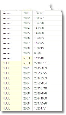 The result looks weird. It breaks all the rules, because it has nulls, and the nulls don’t mean ‘Unknown’ either, they mean ‘total’. This takes some getting used-to. This sort of result wasn’t designed for human consumption.
Basically, you can keep tabs on what the total means by seeing which columns are NULL. In the row below the total for the Yemen (39285) you’ll see a null for the country column and the year column, meaning that this is the total for all years and all countries. If you just mentally substitute the word ‘All’ for NULL then you can’t go far wrong. If all this seems bizarre to you, then you can ignore this and use GROUPING() instead to tell you whether the row is a total. In my aggregate table below, I do both just so you can try different approaches. May Codd forgive us for this!
We’ll put the results in a temporary table. In practice, the original data will be much larger, so the saving in time will be much greater. This sort of table is normally called an ‘Aggregate’ table or ‘Aggregation’ table.
|
1 2 3 4 5 6 7 8 9 10 11 12 13 14 15 16 17 18 19 20 21 22 23 24 25 26 27 28 29 30 31 32 |
if exists (select 1 from tempdb.information_schema.tables where table_name like '#OilProducersAggregate%')DROP TABLE #OilProducersAggregate CREATE TABLE #OilProducersAggregate ( country VARCHAR(25), [year] CHAR(4), production INT,--Crude oil production in Thousand Barrels AvgProduction INT,--Average Monthly production (Thousand Barrels) MaxInsertionDate DateTime, [CountryGrouping] INT, --is this an aggregation row [YearGrouping] INT, --is this an aggregation row ) INSERT INTO #OilProducersAggregate (Country, [Year], production, AvgProduction, MaxInsertionDate,CountryGrouping,YearGrouping) SELECT [country], [year]=DATENAME(year,Date), [production]=SUM(TBPD*Datediff(Day,Date,DateAdd(month,1,Date))), [AvgProduction]=AVG(TBPD*Datediff(Day,Date,DateAdd(month,1,Date))), [MaxInsertionDate]=max(insertionDate), [CountryGrouping]=GROUPING(country), [YearGrouping]=GROUPING(DATENAME(year,Date)) FROM CrudeOilProduction GROUP BY country,DATENAME(year,Date) WITH CUBE |
Something that is more understandable comes from using the results of a CUBE with a PIVOT.
|
1 2 3 4 5 6 7 8 9 10 11 12 |
SELECT country, [2001], [2002], [2003], [2004], [2005], [2006], [2007], [2008], [2009] AS [2009 (part)], [Total] FROM ( SELECT [country]=COALESCE(country,'All'),--to get a row labelled 'All' [year]=COALESCE([year],'Total'),--to get a column headed 'Total' [production], [Countrygrouping] FROM #OilProducersAggregate--just 351 rows. No sweat ) s PIVOT (SUM(production) FOR [Year] IN ([2001], [2002], [2003], [2004], [2005], [2006], [2007], [2008],[2009], [Total])) AS p ORDER BY [Countrygrouping],country |
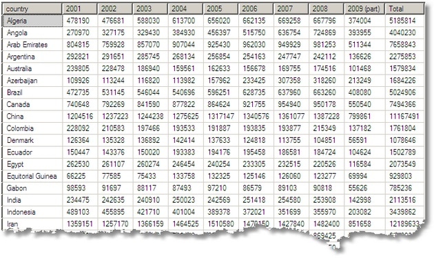
Notice that I”m using the GROUPING() information stored in the aggregate table to sort the order of the rows so that the total is where it should be on the bottom line.
With a minor modification, we will give you the average monthly production. Notice we can still use the ‘SUM’ function for the pivot, since the is only one row for each cell.
|
1 2 3 4 5 6 7 8 9 10 11 12 |
SELECT country, [2001], [2002], [2003], [2004], [2005], [2006], [2007], [2008],[2009] AS [2009 (part)], [Total] FROM ( SELECT [country]=COALESCE(country,'All'),--to get a row labelled 'All' [year]=COALESCE([year],'Total'),--to get a column headed 'Total' [production]=avgProduction, [Countrygrouping] FROM #OilProducersAggregate--just 351 rows. No sweat ) s PIVOT (SUM(production) FOR [Year] IN ([2001], [2002], [2003], [2004], [2005], [2006], [2007], [2008],[2009], [Total])) AS p ORDER BY [Countrygrouping],country |
If you don’t have the pivot operator, (SQL Server 2005 or above) it doesn’t really matter. The old ways were almost as good though more verbose.
|
1 2 3 4 5 6 7 8 9 10 11 12 13 14 15 16 17 18 19 20 21 22 23 24 |
SELECT country, [2001]=SUM(CASE WHEN year ='2001' THEN production ELSE 0 END), [2002]=SUM(CASE WHEN year ='2002' THEN production ELSE 0 END), [2003]=SUM(CASE WHEN year ='2003' THEN production ELSE 0 END), [2004]=SUM(CASE WHEN year ='2004' THEN production ELSE 0 END), [2005]=SUM(CASE WHEN year ='2005' THEN production ELSE 0 END), [2006]=SUM(CASE WHEN year ='2006' THEN production ELSE 0 END), [2007]=SUM(CASE WHEN year ='2007' THEN production ELSE 0 END), [2008]=SUM(CASE WHEN year ='2008' THEN production ELSE 0 END), [2009 (part)]=SUM(CASE WHEN year ='2009' THEN production ELSE 0 END), [Total]=SUM(CASE WHEN year ='Total' THEN production ELSE 0 END) FROM ( SELECT [country]=COALESCE(country,'All'),--to get a row labelled 'All' [year]=COALESCE([year],'Total'),--to get a column headed 'Total' [production]=avgProduction,--just change this line to get the totel production. [Countrygrouping] FROM #OilProducersAggregate--just 351 rows. No sweat ) s GROUP BY country ORDER BY MAX([Countrygrouping]),country |
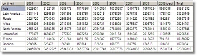
“very nice but what we actually wanted was a breakdown by continent”
–“Right away, Sir!”
We have a slight problem because the original data had an ‘other’ field for countries. We get over this by doing a left outer join with our list of regions, and pick up the unmatched countries) as ‘unmatched’ neatly sidestepping the fact that total lines will also have a null in the country column by checking the ‘grouping’ column*/
|
1 2 3 4 5 6 7 8 9 10 11 12 13 14 15 16 17 18 19 |
SELECT continent, [2001], [2002], [2003], [2004], [2005], [2006], [2007], [2008], [2009] AS [2009 (part)], [Total] FROM ( SELECT [continent]=CASE WHEN GROUPING(continent)=0 AND continent IS NULL THEN 'unclassified' WHEN GROUPING(continent)=1 THEN 'All' ELSE continent END, [year]=COALESCE([year],'Total'), [production]=SUM(production), [grouping]=GROUPING(continent) FROM #OilProducersAggregate s LEFT OUTER JOIN regions o ON o.country = s.country WHERE s.YearGrouping=0 AND countryGrouping=0 GROUP BY continent,year WITH CUBE) g PIVOT (SUM(production) FOR [Year] IN ([2001], [2002], [2003], [2004], [2005], [2006], [2007], [2008], [2009], [Total])) AS p ORDER BY [grouping],total DESC |
–‘What about the breakdown by Opec/Non opec countries? And rotate it the other way while you’re about it’
‘No problem, boss’
|
1 2 3 4 5 6 7 8 9 10 11 12 |
SELECT [year]=COALESCE([year],'Total'), [OPEC]=SUM(CASE WHEN opec_member=1 THEN production ELSE 0 END), [Non-OPEC]=SUM(CASE WHEN opec_member=0 THEN production ELSE 0 END), [Both]=SUM(production) FROM #OilProducersAggregate s LEFT OUTER JOIN regions o ON o.country = s.country WHERE s.YearGrouping=0 AND countryGrouping=0 GROUP BY year WITH CUBE ORDER BY GROUPING(year),CONVERT(INT,year) |
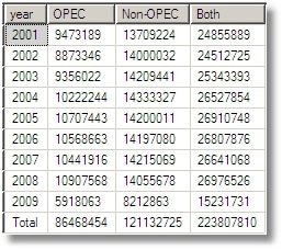
We could have used Rollup, instead of cube, for this last report …
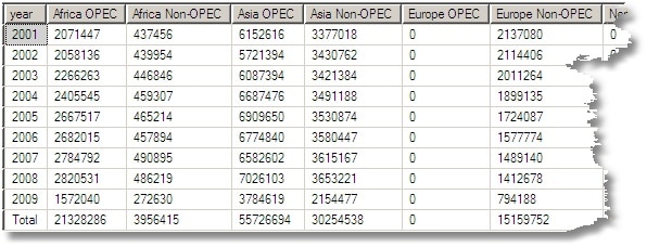
…and a simple modification will get you the yearly breakdown, OPEC vs non OPEC
|
1 2 3 4 5 6 7 8 9 10 11 12 13 14 15 16 17 18 19 20 21 22 23 24 25 26 27 28 29 30 31 32 33 34 35 36 37 38 39 40 41 42 43 |
SELECT [year]=COALESCE([year],'Total'), [Africa OPEC]=SUM(CASE WHEN opec_member=1 AND continent ='Africa' THEN production ELSE 0 END), [Africa Non-OPEC]=SUM(CASE WHEN opec_member=0 AND continent ='Africa' THEN production ELSE 0 END), [Asia OPEC]=SUM(CASE WHEN opec_member=1 AND continent ='Asia' THEN production ELSE 0 END), [Asia Non-OPEC]=SUM(CASE WHEN opec_member=0 AND continent ='Asia' THEN production ELSE 0 END), [Europe OPEC]=SUM(CASE WHEN opec_member=1 AND continent ='Europe' THEN production ELSE 0 END), [Europe Non-OPEC]=SUM(CASE WHEN opec_member=0 AND continent ='Europe' THEN production ELSE 0 END), [North America OPEC]=SUM(CASE WHEN opec_member=1 AND continent ='North America' THEN production ELSE 0 END), [North America Non-OPEC]=SUM(CASE WHEN opec_member=0 AND continent ='North America' THEN production ELSE 0 END), [South America OPEC]=SUM(CASE WHEN opec_member=1 AND continent ='Latin America and the Caribbean' THEN production ELSE 0 END), [South America Non-OPEC]=SUM(CASE WHEN opec_member=0 AND continent ='Latin America and the Caribbean' THEN production ELSE 0 END), [Oceania OPEC]=SUM(CASE WHEN opec_member=1 AND continent ='Oceania' THEN production ELSE 0 END), [Oceania Non-OPEC]=SUM(CASE WHEN opec_member=0 AND continent ='Oceania' THEN production ELSE 0 END), [Russia OPEC]=SUM(CASE WHEN opec_member=1 AND continent ='Russia' THEN production ELSE 0 END), [Russia Non-OPEC]=SUM(CASE WHEN opec_member=0 AND continent ='Russia' THEN production ELSE 0 END), [OPEC]=SUM(CASE WHEN opec_member=1 THEN production ELSE 0 END), [Non-OPEC]=SUM(CASE WHEN opec_member=0 THEN production ELSE 0 END), [all]=SUM(production) FROM #OilProducersAggregate s LEFT OUTER JOIN regions o ON o.country = s.country WHERE s.YearGrouping=0 AND countryGrouping=0 GROUP BY year WITH ROLLUP ORDER BY GROUPING(year),CONVERT(INT,year) |
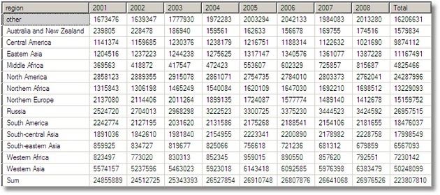
|
1 2 3 4 5 6 7 8 9 10 11 12 13 14 15 16 17 18 19 20 21 22 23 24 25 26 27 28 29 30 |
SELECT COALESCE(region,'other') AS region, [2001]=SUM(CASE WHEN year ='2001' THEN production ELSE 0 END), [2002]=SUM(CASE WHEN year ='2002' THEN production ELSE 0 END), [2003]=SUM(CASE WHEN year ='2003' THEN production ELSE 0 END), [2004]=SUM(CASE WHEN year ='2004' THEN production ELSE 0 END), [2005]=SUM(CASE WHEN year ='2005' THEN production ELSE 0 END), [2006]=SUM(CASE WHEN year ='2006' THEN production ELSE 0 END), [2007]=SUM(CASE WHEN year ='2007' THEN production ELSE 0 END), [2008]=SUM(CASE WHEN year ='2008' THEN production ELSE 0 END), [Total]=SUM(production) FROM #OilProducersAggregate s LEFT OUTER JOIN regions o ON o.country = s.country WHERE s.YearGrouping=0 AND countryGrouping=0 GROUP BY region UNION ALL SELECT 'Sum', [2001]=SUM(CASE WHEN year ='2001' THEN production ELSE 0 END), [2002]=SUM(CASE WHEN year ='2002' THEN production ELSE 0 END), [2003]=SUM(CASE WHEN year ='2003' THEN production ELSE 0 END), [2004]=SUM(CASE WHEN year ='2004' THEN production ELSE 0 END), [2005]=SUM(CASE WHEN year ='2005' THEN production ELSE 0 END), [2006]=SUM(CASE WHEN year ='2006' THEN production ELSE 0 END), [2007]=SUM(CASE WHEN year ='2007' THEN production ELSE 0 END), [2008]=SUM(CASE WHEN year ='2008' THEN production ELSE 0 END), total=SUM(production) FROM #OilProducersAggregate s WHEREs.YearGrouping=0 ANDcountryGrouping=0 |
So why did we put an insertion date into the raw and aggregate data? This was so we can re-aggregate all or part of the data when something gets changed. I must admit that, for an accounting system, i’d want to know why, rather than just redo the aggregation, but in this example we’d just re-aggregate if this SQL produces a non-zero result.
|
1 2 3 4 5 6 7 |
SELECT DISTINCT s.year, s.country FROM CrudeOilProduction c INNER JOIN #OilProducersAggregate s ON s.country =c.country AND s.[year]=DATENAME(year,c.Date) WHERE insertionDate>MaxInsertionDate |
Where you have many millions of rows, and only want to alter any totals that have changed, the logic can get quite tricky as you have to redo all the dependent totals without recalculating everything, and the logic for a cube can get very messy indeed, way too much to describe in this article.
Conclusions
Well, once you have a cube in place, there is a great deal of reporting you can do with it without having to go back to the raw data. Although the CUBE operator is now made to look pretty archaic when compared with what SSAS offers, there is still a lot of life left in the technique for doing ad-hoc reports on-demand without the overhead of SSAS. For supplying data to Excel or reporting services, it can be a godsend.
Pivoting and un-pivoting is simple to do. In another article, The Cross-Tab Pivot Table Workbench, Robyn and I have shown how to do a variety of such things, and even how to go into mass production with pivot tables without bothering with reporting services,
The other conclusion from the data is that, at the time of writing, we have a lot of work to do in reducing our dependence on fossil fuel. The figures for oil production show that the downturn hasn’t made a huge difference to demand! Never mind. In Simple-Talk’s offices, they’ve changed the light-bulb for a fluorescent, in a bid to save the planet.
Load comments