There are many new features in SQL Server 2022. In relation to T-SQL querying, there are a few as well and they usually are left for last in face of many other new optimization features.

Sample scenario

These samples are built on the AdventureWorksDW2019 database installed in a SQL Server 2022 CTP 2.

Date_Bucket

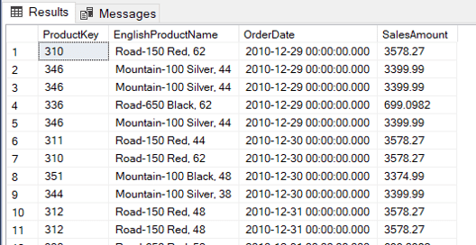
Let’s first consider a sample query. The following query shows information about internet sales and products.

 

The Date_Bucket function, as the name implies, calculates date buckets of one specific size. Given a date and the bucket size, the function will return the start date of the bucket containing the date.

This is very useful to classify the facts in our data in groups according a date bucket. For example, we can create 2 weeks bucket, 2 months bucket and so on. The date bucket function is useful for grouping on these scenarios.

For example, based on the query above, let’s create a 1 week date bucket to group the product sales.

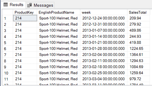
If we change the size of the bucket to 2 weeks, instead of one, you may notice on the following image the dates organized for each two weeks.

The calculation of the buckets needs a starting point. This is an optional parameter. When we don’t specify the starting point, the calculation starts on 01/01/1900. That’s how it was calculates on the previous two queries.

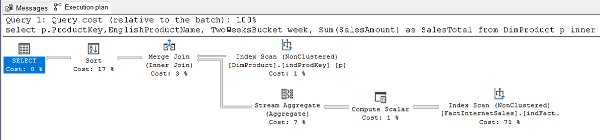
There is no surprise the Date_Bucket expression is not a SARG. As you may notice on the execution plan below, the index operations are all SCAN.

 

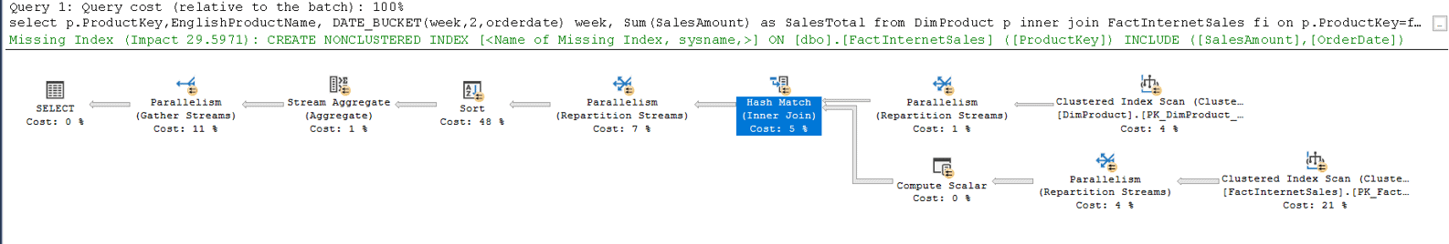
The query plan complains about some missing indexes. Let’s create them first and analyse the impact of Date_bucket isolated from other needs in the query.

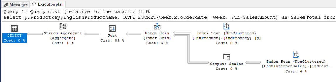
After these indexes are created, the query plan will be like this one below:

 

Let’s execute the follow statements followed by the query execution to get a clean statistics. Don’t do this in a production environment.

SQL Server parse and compile time:
CPU time = 0 ms, elapsed time = 55 ms.

(3959 rows affected)
Table ‘Worktable’. Scan count 0, logical reads 0, physical reads 0, page server reads 0, read-ahead reads 0, page server read-ahead reads 0, lob logical reads 0, lob physical reads 0, lob page server reads 0, lob read-ahead reads 0, lob page server read-ahead reads 0.
Table ‘FactInternetSales’. Scan count 1, logical reads 345, physical reads 0, page server reads 0, read-ahead reads 344, page server read-ahead reads 0, lob logical reads 0, lob physical reads 0, lob page server reads 0, lob read-ahead reads 0, lob page server read-ahead reads 0.
Table ‘DimProduct’. Scan count 1, logical reads 6, physical reads 1, page server reads 0, read-ahead reads 11, page server read-ahead reads 0, lob logical reads 0, lob physical reads 0, lob page server reads 0, lob read-ahead reads 0, lob page server read-ahead reads 0.

SQL Server Execution Times:
CPU time = 47 ms, elapsed time = 112 ms.

There are two solutions to improve the performance with the Date_Bucket function:

• If the Buckets match with information in a date dimension, using the date dimension instead of date_bucket will perform better. Leaves the date_bucket function for buckets which don’t match with information in the date dimension.
• If the bucket is used very often, create a calculated field and uses it in an index.

Considering the indexes we created before, the code to create and use the calculated field will be like this:

The new query will need to use the calculated field. The new query plan changes the location of the stream aggregate and the cost of the SORT is very reduced. We need to check the statistics and time to compare the new query with the old one.

SQL Server parse and compile time:
CPU time = 31 ms, elapsed time = 64 ms.

(3959 rows affected)
Table ‘Worktable’. Scan count 0, logical reads 0, physical reads 0, page server reads 0, read-ahead reads 0, page server read-ahead reads 0, lob logical reads 0, lob physical reads 0, lob page server reads 0, lob read-ahead reads 0, lob page server read-ahead reads 0.
Table ‘FactInternetSales’. Scan count 1, logical reads 405, physical reads 0, page server reads 0, read-ahead reads 409, page server read-ahead reads 0, lob logical reads 0, lob physical reads 0, lob page server reads 0, lob read-ahead reads 0, lob page server read-ahead reads 0.
Table ‘DimProduct’. Scan count 1, logical reads 6, physical reads 1, page server reads 0, read-ahead reads 11, page server read-ahead reads 0, lob logical reads 0, lob physical reads 0, lob page server reads 0, lob read-ahead reads 0, lob page server read-ahead reads 0.

SQL Server Execution Times:
CPU time = 15 ms, elapsed time = 68 ms.

The CPU time and Elapsed Time improved a lot from the original query.

You can read more about Date_Bucket here

Window Expression

The window functions and OVER expressions are present since SQL Server 2018. Now we have a new expression to make it easier to write these queries.

The OVER expression allows us to retrieve detail data about the rows and aggregated data at the same time.

For example, considering the previous example using date_bucket, we can bring the details of each transaction and the total of the week bucket. We also can make a percentage calculation comparing each transaction with the bucket’s total

The query will be like this:

 

The new WINDOW expression allows us to simplify the query by writing the WINDOW expression once, in the end of the query, and referencing it where it’s needed, even more than once.

Using the WINDOW expression, the query will be like this:

 

The queries will have the same execution plan, the new syntax will not affect the execution, it will only make them easier to read.

You can read more about the window exprpession here: https://docs.microsoft.com/en-us/sql/t-sql/queries/select-window-transact-sql?WT.mc_id=DP-MVP-4014132&view=sql-server-ver16 

LEAST and GREATEST function

These new functions are used to find the smallest and biggest value in a set of values. They are not intended to be used in a set of records, for this we have the MAX and MIN aggregation functions. LEAST and GREATEST are intended to be used in a set of values, for example, a set of fields.

Let’s build one useful example for these functions. We can use the PIVOT statement in SQL Server to transform a rows into columns, comparing the sales of the products in a single quarter, for example.

A regular query without using the PIVOT would be like this:

Using the PIVOT on this query we can turn the months into columns:

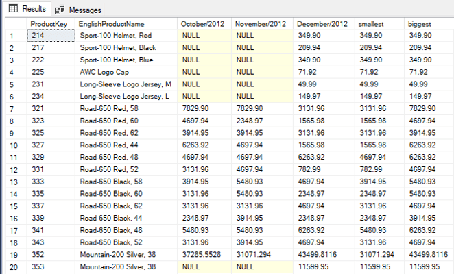
This is a great example to use LEAST and GREATEST to find the smallest and biggest values in a quarter:

 

Summary

These are only 3 of the interesting T-SQL improvements in SQL Server 2022