
Until recently, most of the talk about tabular data revolved around PowerPivot, an Excel add-in that brings powerful in-memory data crunching to the spreadsheet environment. Creating a tabular database in PowerPivot, and by extension, within Excel, is a fairly prescribed process that involves retrieving data from one or more data sources-most notably SQL Server databases-and creating one or more tables based on that data.
Despite all the attention paid to PowerPivot and its tabular databases, there has been relatively little focus on how to retrieve tabular data directly from a SQL Server Analysis Services (SSAS) instance into Excel, whether through PowerPivot or directly into a workbook.
In this article, we explore how to use Excel to view and retrieve data from an SSAS tabular database. This is the third article in a series about SSAS tabular data. In the last article, “Using DAX to retrieve tabular data,” we discussed how to create Data Analysis Expressions (DAX) statements to retrieve tabular data, working from within SQL Server Management Studio (SSMS) to run our queries against an SSAS tabular instance. Some of what was covered in that article will apply to retrieving data from within Excel.
For this article, I provide a number of examples of how to import tabular data into Excel. The examples pull data from the AdventureWorks Tabular Model SQL 2012 database, available as a SQL Server Data Tools (SSDT) tabular project from the AdventureWorks CodePlex site. On my system, I’ve implemented the database on a local instance of SSAS 2012 in tabular mode.
Viewing Browsed Data in Excel
We got a taste of how to browse data from within SSMS in the first article of this series, “Getting Started with the SSAS Tabular Model.” In Object Explorer, right-click the database and then click Browse. When the Browse window appears, you can view a list of database objects and use those objects to retrieve data by dragging them into the main workspace. For example, Figure 1 shows data from the Country Region Name and City columns of the Geography table, as well as from the Internet Total Sales and Internet Total Units measures of the Internet Sales table.
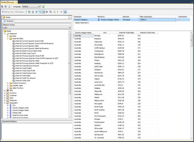
Figure 1: Browsing tabular data in SSMS
Notice in Figure 1 that I also created a filter that limits the amount of data returned. (You define filters in the small windows above the main workspace.) In this case, I eliminated all sales that include the value Bikes in the Category Name column of the Product table. This way, all non-bike merchandise is included in the sales figures.
What’s shown in Figure 1 is pretty much the extent of what you can do in the Browse window in SSMS. To be able to fully drill into the data, you need to use Excel. Starting with SQL Server 2012, Excel is now the de facto tool in SSMS and SSDT for analyzing tabular data. Unfortunately, that means you need Office 2003 or later installed on the same computer where SSMS and SSDT are installed, not a practical solution for everyone. Even so, having Excel installed makes analyzing tabular data a much easier process.
Part of that simplicity lies in the fact that the SSMS Browse window and the SSDT tabular project window both include the Analyze in Excel button on their respective menus. The button launches Excel and let’s you browse the tabular data from within in a pivot table.
When you first click the Analyze in Excel button, you must choose which perspective to open in Excel, as shown in Figure 2. As you might recall from the first article, a perspective represents all or part of the data model. The Model perspective includes all database components.
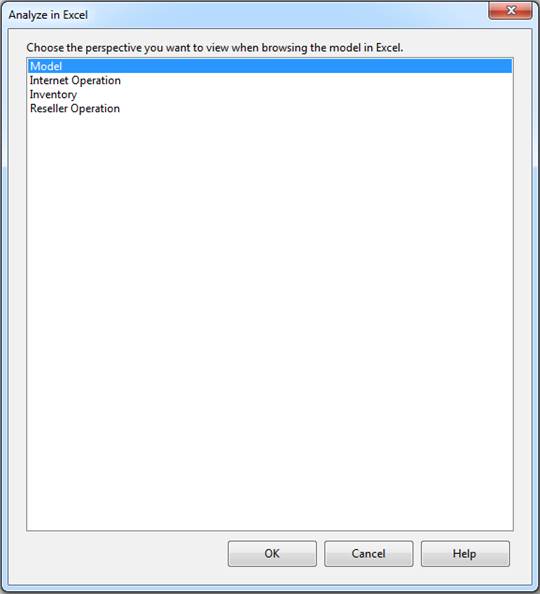
Figure 2: Selecting a perspective when sending data to Excel
Once you’ve selected a perspective, click OK. Excel is launched and opens to a new pivot table that automatically connects to the SSAS tabular data source. Figure 3 shows the pivot table before any data has been added. Notice in the right window you’ll find the PivotTable Field List pane, which contains a list of all your database objects, including tables, columns, and measures.
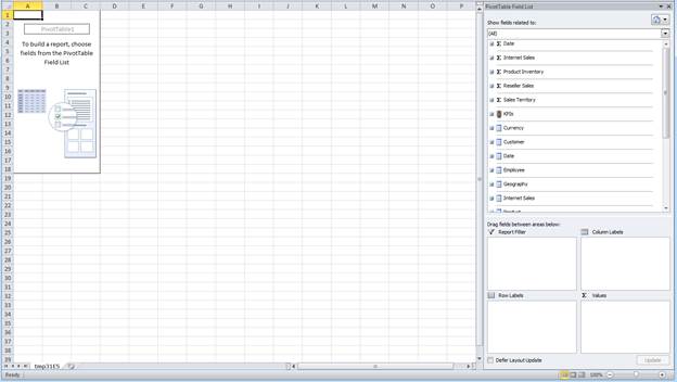
Figure 3: Importing tabular data into an Excel pivot table
To get started with the pivot table, drag the fields and measures you want to include in your report to the Column Labels, Row Labels, and Values panes. The data will then be displayed in the pivot table. You can also create filters by dragging fields to the Report Filter pane. Figure 4 shows the pivot table after I added numerous database objects. Many of these objects are the same columns and measures that were added to the Browse window shown in Figure 1, except that now I also break down the sales by years.
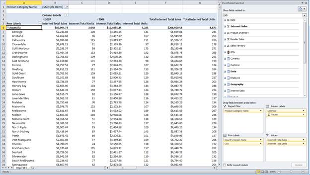
Figure 4: Working with tabular data in an Excel pivot table
To configure the pivot table shown in Figure 4, I added the following database objects to the specified configuration panes in the right window:
- The
Country Region Namecolumn from theGeographytable to theRow Labelspane. - The
Citycolumn from theGeographytable to theRow Labelspane. - The
Yearcolumn (from the Calendar hierarchy) of theDatetable to theColumn Labelspane. - The
Internet Total Salesmeasure from the Internet Salestable to theValuespane. - The
Internet Total Unitsmeasure from theInternet Salestable to theValuespane. - The
Product Category Namecolumn from theProducttable to theReport Filterpane.
Once you’ve set up your pivot table, you can play around with the data however you want. For example, you can drill down into the year values or view only the country totals without viewing the cities. You can also find rollups for each category of data. Plus, you can filter data based on the values in the Product Category Name column. Keep in mind, however, that this article is by no means a tutorial on how to work with Excel pivot tables. For that, you need to check out the Excel documentation. SSMS and SSDT make it easy to view the data in Excel, but it’s up to you to derive meaning from what you find.
Importing Data into an Excel Pivot Table
Not everyone will have SSMS or SSDT installed on their systems, but they might still need to access an SSAS instance to retrieve tabular data. In that case, they can establish their own connection to the tabular database (assuming they have the necessary permissions) and import the data into a pivot table, just as we saw above.
To connect to a tabular database from within Excel, go to the Data tab, click the From Other Sources button, and then click From Analysis Services. When the Data Connection Wizard appears, type the instance name and any necessary logon credentials, as shown in Figure 5. (In my case, I used Windows Authentication.)
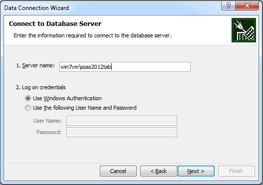
Figure 5: Connecting to an SSAS instance in tabular mode
Click Next to advance to the Select Database and Table page, shown in Figure 6. Here you select the database you want to connect to and the specific perspective. Once again, I’ve selected Model in order to retrieve all the database components. (As you’ve probably noticed, Microsoft is somewhat inconsistent in its interfaces when it comes to referring to perspectives in a tabular database. Sometimes they’re referred to as cubes, sometimes perspective, and sometimes Model is referred to as a cube and the other components as perspectives. I’m not sure how Table fits into the picture.)
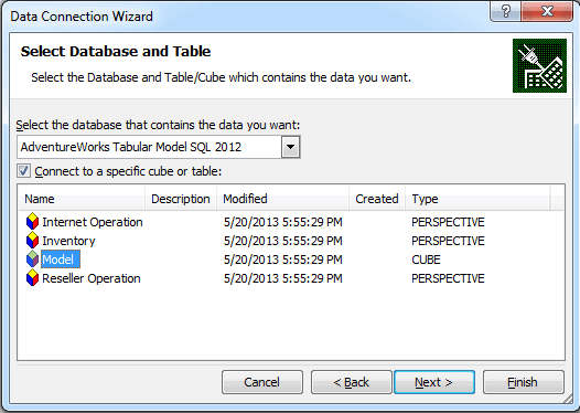
Figure 6: Selecting a perspective when connecting to tabular data
After you’ve selected your database and perspective, click Next to advance to the Save Data Connection File and Finish page, shown in Figure 7. Here you can provide a name for the data connection file (an .odc file), a description of the connection, and a friendly name for the connection.
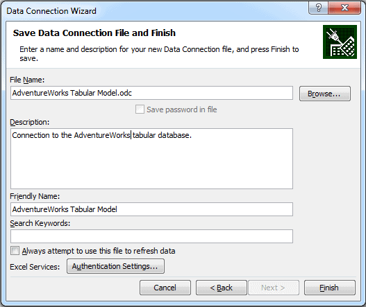
Figure 7: Creating a data connection file in Excel
Once you’ve supplied the necessary information, click Finish. You’ll then be presented with the Import Data dialog box, as shown in Figure 8. You can choose whether to create a pivot table, a pivot table and pivot chart, or the data connection only. You can also choose to use the existing worksheet or open a new one.
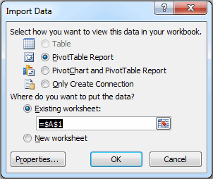
Figure 8: Importing tabular data into a pivot table
You might have noticed that the Table option is grayed out. When importing tabular data in this way, Excel is very picky. Either you use a pivot table (and pivot chart, if you want) or nothing at all. You cannot import the data into a set of tables. However, there is a way to work around the default behavior, which we cover in the following section.
But for now, stick with the default options (those shown in Figure 8), and click OK. You’ll then be presented with a new pivot table and the PivotTable Field List pane, with all the tables and their columns and measures listed, similar to what is shown in Figure 3. You can then work with that data to create a report just like we did earlier.
Using DAX to Import Data into Excel
To import tabular data into a regular Excel table, rather than a pivot table, we can create a DAX expression that pulls in exactly the data we need. We start by creating a data connection, just as we did in the last section. Once again, launch the Data Connection Wizard and follow the prompts. When you get to the Save Data Connection File and Finish page, provide a file name, description, and friendly name. But keep all the names simple because we’ll be referencing them later in the process and we want to make sure everything is easy to find. Figure 9 shows the names I used to set up the data connection on my system.
Figure 9: Creating a data connection file in Excel
When you click Finish, you’ll again be presented with the Import Data dialog box. This time around, select the option Only Create Connection, as shown in Figure 10. We don’t want to pull in any data just yet. We just want to establish how we’ll be connecting to the tabular database. Click OK to finish creating the connection.
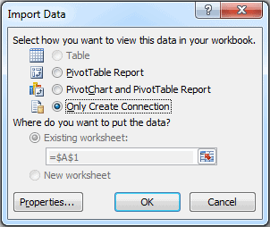
Figure 10: Creating a data connection without creating a pivot table
The next step is to locate the data connection file we just created so we can edit it. On my system, I had named the file aw_query.odc, and I found it in the My Documents/My Data Sources folder associated with my user account.
When editing the connection file, which we can do in Notepad, we want to modify the default settings so we can use a DAX query to retrieve the data. To achieve this, we need to modify two lines, the CommandType and CommandText elements, which are highlighted in the following HTML:
|
1 2 3 4 5 6 7 8 9 10 11 12 13 14 15 16 17 18 19 20 21 22 23 24 25 26 27 28 29 30 31 32 33 |
<head> <meta http-equiv=Content-Type content="text/x-ms-odc; charset=utf-8"> <meta id="ProgId" content=ODC.Cube> <meta id="SourceType" content=OLEDB> <meta id="Catalog" content="AdventureWorks Tabular Model SQL 2012"> <meta id="Table" content=Model> <title>AdventureWorks query</title> <xml id="docprops><o:DocumentProperties"> xmlns:o="urn:schemas-microsoft-com:office:office" xmlns="http://www.w3.org/TR/REC-html40"> <o:Description>Generate DAX statement to retrieve table from AdventureWorks database.</o:Description> <o:Name>AdventureWorks query</o:Name> </o:DocumentProperties> </xml> <xml id="msodc><odc:OfficeDataConnection"> xmlns:odc="urn:schemas-microsoft-com:office:odc" xmlns="http://www.w3.org/TR/REC-html40"> <odc:Connection odc:Type="OLEDB"> <odc:ConnectionString>Provider=MSOLAP.4;Integrated Security=SSPI;Persist Security Info=True;Data Source=win7vm\ssas2012tab;Initial Catalog=AdventureWorks Tabular Model SQL 2012</odc:ConnectionString> <odc:CommandType>Cube</odc:CommandType> <odc:CommandText>Model</odc:CommandText> </odc:Connection> </odc:OfficeDataConnection> </xml> <style> <!-- .ODCDataSource { behavior: url(dataconn.htc); } --> </style> </head> |
The HTML shown here is the head section of the data connection file. For the CommandType element, replace the value Cube with the value query. This tells Excel to let us pass a query in through our data connection, rather than having to identify a specific perspective.
For the CommandText element, replace the value Model with a DAX statement that retrieves data into a single result set. For this example, I pulled the following query from the last article in this series (so return to that article for an explanation):
|
1 2 3 4 5 6 7 8 9 10 11 12 13 14 15 16 17 18 19 20 21 22 23 |
evaluate ( filter ( addcolumns ( summarize ( 'Internet Sales', 'Product'[Product Name], 'Product Subcategory'[Product Subcategory Name], 'Product Category'[Product Category Name], 'Date'[Calendar Year] ), "Total Sales Amount", calculate(sum('Internet Sales'[Sales Amount])), "Total Cost", calculate(sum('Internet Sales'[Total Product Cost])) ), 'Date'[Calendar Year] > 2006 ) ) order by 'Product'[Product Name], 'Date'[Calendar Year] |
You can use a different query, of course, whatever serves your needs. The goal is to retrieve the data into a single table that you can view in an Excel worksheet, just like any other worksheet. After you modify the HTML in the data connection file, the head section should look similar to the following:
|
1 2 3 4 5 6 7 8 9 10 11 12 13 14 15 16 17 18 19 20 21 22 23 24 25 26 27 28 29 30 31 32 33 34 35 36 37 38 39 40 41 42 43 44 45 46 47 48 49 50 51 52 53 54 55 56 57 |
<head> <meta http-equiv=Content-Type content="text/x-ms-odc; charset=utf-8"> <meta id="ProgId" content=ODC.Cube> <meta id="SourceType" content=OLEDB> <meta id="Catalog" content="AdventureWorks Tabular Model SQL 2012"> <meta id="Table" content=Model> <title>AdventureWorks query</title> <xml id="docprops><o:DocumentProperties"> xmlns:o="urn:schemas-microsoft-com:office:office" xmlns="http://www.w3.org/TR/REC-html40"> <o:Description>Generate DAX statement to retrieve table from AdventureWorks database.</o:Description> <o:Name>AdventureWorks query</o:Name> </o:DocumentProperties> </xml> <xml id="msodc><odc:OfficeDataConnection"> xmlns:odc="urn:schemas-microsoft-com:office:odc" xmlns="http://www.w3.org/TR/REC-html40"> <odc:Connection odc:Type="OLEDB"> <odc:ConnectionString>Provider=MSOLAP.4;Integrated Security=SSPI;Persist Security Info=True;Data Source=win7vm\ssas2012tab;Initial Catalog=AdventureWorks Tabular Model SQL 2012</odc:ConnectionString> <odc:CommandType>query</odc:CommandType> <odc:CommandText> evaluate ( filter ( addcolumns ( summarize ( 'Internet Sales', 'Product'[Product Name], 'Product Subcategory'[Product Subcategory Name], 'Product Category'[Product Category Name], 'Date'[Calendar Year] ), "Total Sales Amount", calculate(sum('Internet Sales'[Sales Amount])), "Total Cost", calculate(sum('Internet Sales'[Total Product Cost])) ), 'Date'[Calendar Year] > 2006 ) ) order by 'Product'[Product Name], 'Date'[Calendar Year] </odc:CommandText> </odc:Connection> </odc:OfficeDataConnection> </xml> <style> <!-- .ODCDataSource { behavior: url(dataconn.htc); } --> </style> </head> |
I highlighted the new code to make it easier to pick out. I also laid out the DAX statement so it’s more readable. However, you don’t need to break it apart in this way to add it into the file. (The parser ignores the extra whitespace and line breaks.)
After you save and close the data connection file, it’s time to verify what you’ve done. In Excel, go to the Data tab and click Existing Connections. When the Existing Connections dialog box appears, double-click the connection you just edited. It will be listed under its friendly name, not the file name. On my system, the connection’s friendly name is AdventureWorks query. This launches the Import Data dialog box, shown in Figure 11. Notice that this time around, the Table option is available and selected.
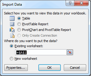
Figure 11: Importing tabular data into an Excel table
Click OK to close the Import Data dialog box. A table will appear, populated with the data retrieved through the DAX statement, as shown in Figure 11. You can then sort through the data and create any necessary filters.
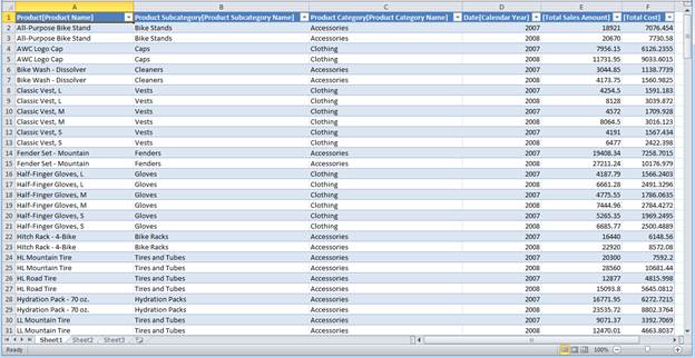
Figure 12: Working with tabular data in an Excel table
When you’re working in a table based on tabular data, you can modify the connection associated with the current workbook. Doing so, however, severs its relationship to the original .odc data connection file. Instead, your changes are saved to the connection specifically associated with that workbook. The .odc file remains unchanged. Updating the connection in this way lets you modify the DAX statement, change the connection string, or configure other properties.
To modify the workbook’s connection, go to the Data tab and click Connections. This launches the Workbook Connections dialog box, shown in Figure 13. Here you should find the connection you created earlier. On my system, this is AdventureWorks query.
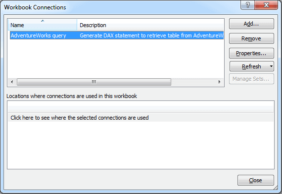
Figure 13: Viewing the data connections associated with an Excel workbook
Next, we want to access the connection’s properties. Make sure the connection is selected (in case you have more than one connection listed), and then click Properties. This launches the Connection Properties dialog box. Go to the Definition tab and expand the dialog box as necessary to easily view the DAX statement. Figure 14 shows what the dialog box looks like on my system.
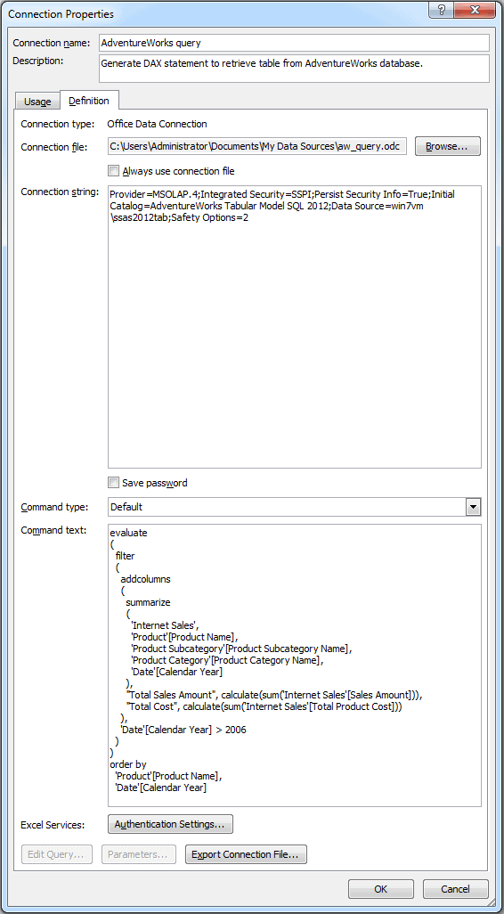
Figure 14: Viewing the properties of an Excel data connection
Chances are, when you open the dialog box, the DAX statement will be difficult to read. The statement shown in Figure 14 is what it looked like after I organized things a bit for readability. The changes I made have no impact on the statement itself.
You can modify the DAX statement or connection string as necessary (or any other properties, for that matter). To save you changes, click OK. You’ll then be presented with an Excel message box warning you that you are about to sever ties with the original data connection file, as shown in Figure 15. That’s not a problem, though, because your updated connection information will be saved with the workbook when you save it.
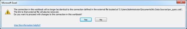
Figure 15: Severing ties between a data connection and its source file
You can now update you connection as often as you like. You should not receive this warning going forward. You can also use the existing .odc connection to easily add other tables to your workbook. To do so, add a new worksheet, connect to the data source via the .odc connection, and then modify the connection properties by adding a different DAX statement. (You can also rename the connection as necessary.) That way you can create a workbook that contains numerous worksheets that each includes an imported table from a tabular data source.
Using DAX to Import Data into PowerPivot
Up to this point, I’ve shied away from discussing PowerPivot in too great of detail, mostly because it’s already received so much press. But one issue that’s received little attention is how you retrieve data from an SSAS tabular instance into PowerPivot.
Surprisingly, the functionality is somewhat limited. You would expect-or at least I would expect-that I could import all the tables, along with their columns and measures, in a single connection, just as I can do with an Excel pivot table or a SQL Server database in PowerPivot. But that doesn’t appear to be the case. The only option I can find for importing tabular data directly into PowerPivot is one table at a time, just like we saw with Excel tables. However, doing so in PowerPivot is a bit easier.
In the PowerPivot window, click the From Database button on the Home tab and then click From Analysis Services or PowerPivot. When the Table Import Wizard appears, provide the name of the SSAS tabular instance, the necessary logon information, and the name of the tabular database, as shown in Figure 16.
Figure 16: Defining a data connection to an SSAS tabular database
Don’t forget, you can also provide a friendly connection name. And it’s always a good idea to test your connection. When you’re finished, click Next.
The next page in the wizard is Specify a MDX Query. As with SSMS or your Excel data connections, you can specify a DAX query rather than a Multidimensional Expressions (MDX) query. We’ll go with DAX. Figure 17 shows the page with the same query we used in the previous section. You can use the Validate option to check your statement, which seems to work with DAX, unlike the Design option, which seems happier sticking with MDX.
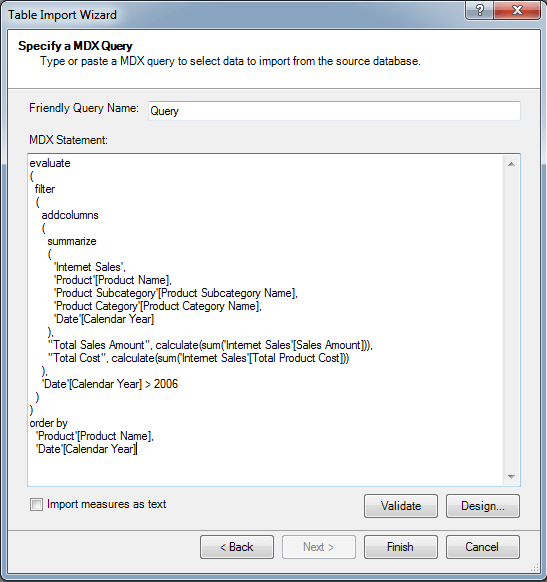
Figure 17: Defining a DAX query to retrieve tabular data from SSAS
After you entered your DAX query (and provided a name for the query, if you like), click Finish to import the data. During this process, you’ll advance to the wizard’s Importing page. If the data is imported with no problems, you should receive a Success message, as shown in Figure 18.
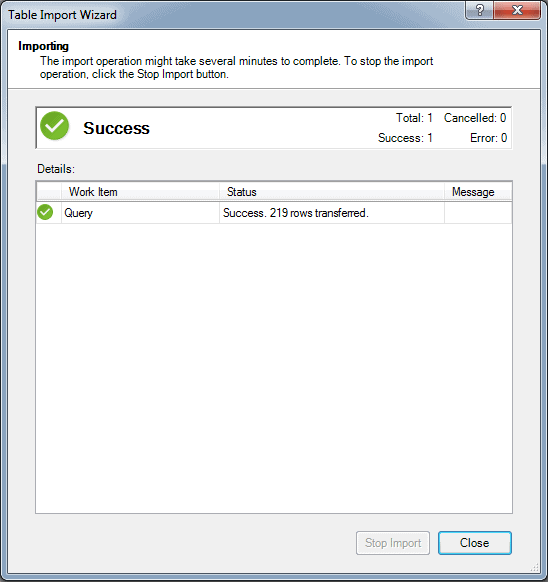
Figure 18: Successfully importing SSAS tabular data into PowerPivot for Excel
Click Close. This will open a new table in the PowerPivot window, with the imported data displayed. Figure 19 shows part of the data returned by the query. If the data is not exactly what you need, you can refine your query as necessary.
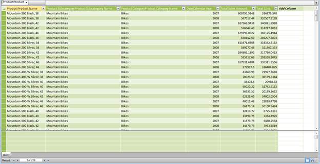
Figure 19: Working with tabular data in PowerPivot for Excel
You can import data into as many tables as you need. You can then create relationships between those tables, assuming you bring in the columns necessary to define those relationships. Not surprisingly, it would be handier to go directly to the source of the data, in this case, the AdventureWorksDW2012 database, so you can retrieve all the tables at once, along with their defined relationships. But you might not have access to that data and have no choice but to be retrieve it directly from the SSAS instance. Or there might be other circumstances that require you to retrieve the data directly from SSAS. Whatever the reason, you now know how it’s done, and once you’ve tried it out, you’ll find it’s a fairly simple operation.
The Excel Connection
As you’ve seen in this article, you have several options for retrieving SSAS tabular data into Excel. You can launch Excel from within SSMS or SSDT. You can import data directly into a pivot table. And you can generate DAX queries to retrieve data into individual Excel and PowerPivot tables. Or instead of DAX, you can generate MDX queries, unless the tabular database has been set up in DirectQuery mode. Regardless, you have a number of options for importing tabular data into Excel. And once you get it there, you have a rich environment for manipulating and analyzing the data, allowing you to create precise and detailed reports in the format you need when you need them, without having to be concerned about SSAS and how the tabular model works.


Load comments