


In this article, part of the “Moving from Python to esProc” series, we’ll look at esProc SPL’s data manipulation capabilities compared to Python.
As you may already know, real-world data rarely arrives in a clean, analysis-ready format. You’ll frequently need to clean messy data, reshape it to suit your analysis needs, merge multiple datasets, and perform complex filtering and calculations before extracting meaningful insights. Luckily, esProc SPL handles these common data manipulation tasks with remarkable elegance and efficiency.
How to clean ‘messy’ data with esProc SPL
Datasets are rarely perfect. Missing values, inconsistent formats, and outliers can significantly impact analysis quality. Let’s look at how esProc SPL handles these data cleaning challenges – often some of the most time-consuming aspects of data analysis.
How to identify and handle missing values in esProc SPL
Missing values occur when data is incomplete. You need to detect and handle them to ensure accurate results. This flowchart illustrates the systematic approach to dealing with missing data in a dataset:
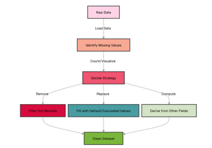
It begins with loading raw data, then moves to identifying missing values through counting and visualization techniques. Once missing values are detected, the process branches into three strategic options: removing records with missing values (which is simple but can lose valuable information), replacing missing values with defaults or calculated substitutes (like means or medians), or computing new values derived from other fields in the dataset.
All three strategies ultimately converge to produce a clean dataset ready for analysis. This flowchart provides a structured decision framework that helps data analysts choose the most appropriate method for handling missing values based on their specific data context and analysis requirements.
The first step in cleaning messy data is identifying missing values. In esProc SPL, missing values are represented as `null`. Let’s start by creating a sample dataset with some missing values:
| A | ||
| 1 | =file(“document/sales.csv”).import@ct() | Sales data with 100 rows |
| 2 | =A1.run(AMOUNT=if(rand()<0.1,null,AMOUNT)) | Randomly set ~10% of AMOUNT values to null |
Now, let’s identify rows with missing values:
| 3 | =A2.select(AMOUNT==null) | Rows with missing AMOUNT |
| 4 | =A3.len() |
The output of A4 will show that we have 10 rows with missing AMOUNT values, which is approximately 10% of our dataset, as expected. Now, let’s count missing values by region:
| 5 | =A2.groups(REGION; count(AMOUNT==null):MISSING_COUNT, count(AMOUNT):TOTAL_COUNT) | Count missing values by region |
This shows the distribution of missing values across regions. Now, let’s handle these missing values using different techniques:
How to remove rows with missing values
| 6 | =A2.select(AMOUNT!=null) | Remove rows with missing AMOUNT |
| 7 | =A6.len() |
The output of A7 shows the number of rows we have after removing the rows with missing AMOUNT values.
How to fill missing values with a constant
| 8 | =A2.derive(ifn(AMOUNT, 0):AMOUNT_FILLED) | Replace nulls with 0 |
How to fill missing values with statistical measures
You can first add the AMOUNT_FILLED field to A2, then fill values directly after grouping. This avoids using new and join, improving performance. This is an SPL-exclusive technique using retained grouped subsets.
| 9 | =A2.derive(:AMOUNT_FILLED) =A2.derive(:AMOUNT_FILLED) |
| 10 | =A9.group(REGION) |
| 11 | =A10.run(a=~.avg(AMOUNT),~.run(AMOUNT_FILLED=ifn(AMOUNT,a))) |
| 12 | =A9.to(5) |
A9: Add an empty AMOUNT_FILLED field to A2.
A10: Group A9 by REGION and retain original record sets within each group. Updating field values in the grouped records will modify the corresponding values in the original table A9.
A11: Iterate through A10. For each group, calculate the average of AMOUNT and store it in a temporary variable a. Then, iterate through the group’s records and assign values to AMOUNT_FILLED. ifn(AMOUNT,a) means: return AMOUNT if it is not null; otherwise, return a.
Simple Talk is brought to you by Redgate Software
How to detect and handle outliers in esProc SPL
Outliers can significantly skew your analysis and lead to incorrect conclusions. Let’s explore how to detect and handle outliers in esProc SPL.
How to identify outliers using Z-score
The Z-score measures how many standard deviations a data point is from the mean. Values with a Z-score greater than 3 or less than -3 are often considered outliers. Since A14 only contains one row, there’s no need to join with A6. You can directly add the Z_SCORE field to A6 and return the final result. The code is as follows:
| 14 | =A6.group(;~.avg(AMOUNT):AVG, sqrt(var@r(~.(AMOUNT))):STD) | Calculate mean and standard deviation |
| 15 | =A6.derive((AMOUNT-A14.AVG)/A14.STD: Z_SCORE) | Join with statistics |
| 16 | =A15.select(abs(Z_SCORE)>2) | Calculate Z-score |
| 17 | =A16.top(-5, Z_SCORE) | Select outliers (Z-score > 2) |
This shows the top outliers based on Z-score. The first two rows have Z-scores greater than 2, indicating they are potential outliers.
How to identify outliers using IQR (interquartile range)
Another common method for detecting outliers is the IQR method, which identifies values below Q1 – 1.5*IQR or above Q3 + 1.5*IQR as outliers:
| 18 | =A6.groups(;median(1:4,AMOUNT):Q1,median(3:4,AMOUNT):Q3) | Calculate Q1 and Q3 |
| 20 | A6.select(AMOUNT<A21.LOWER_BOUND || AMOUNT>A21.UPPER_BOUND) | Select outliers |
| 21 | =A20.top(-5,AMOUNT) | First 5 outliers |
How to handle outliers
Once you’ve identified outliers, you can handle them in several ways, as shown in this flowchart:
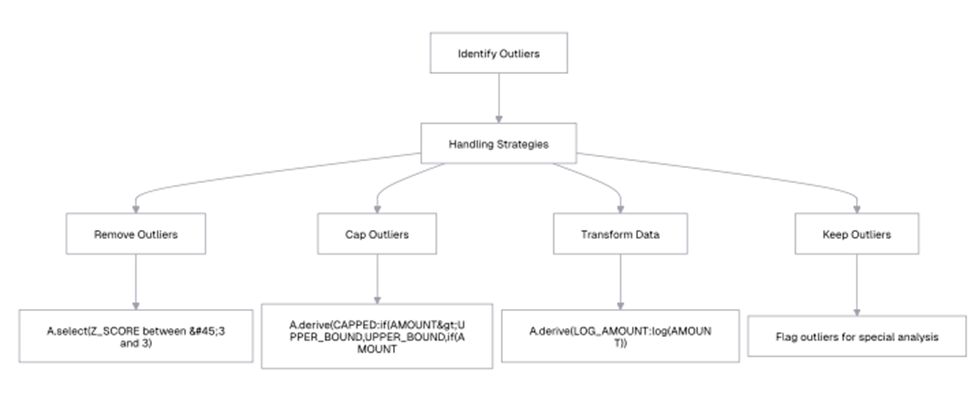
Let’s implement the capping strategy:
| 22 | =A18.derive(AMOUNT_CAPPED:if(AMOUNT>UPPER_BOUND,UPPER_BOUND,if(AMOUNT<LOWER_BOUND,LOWER_BOUND,AMOUNT))) Cap outliers Replace the nested if with: if(AMOUNT>UPPER_BOUND:UPPER_BOUND, AMOUNT<LOWER_BOUND:LOWER_BOUND; AMOUNT) The full line should be: =A22.derive(if(AMOUNT>UPPER_BOUND:UPPER_BOUND, AMOUNT<LOWER_BOUND:LOWER_BOUND; AMOUNT):AMOUNT_CAPPED:) |
| 23 | =A22.select(DATE,REGION,PRODUCT,AMOUNT,AMOUNT_CAPPED) Select relevant columns |
| 24 | =A23.to(5) |
Since our dataset doesn’t have extreme outliers based on the IQR criterion, the capped values are the same as the original values.
How to remove duplicates in esProc SPL
Duplicate records can skew your analysis and lead to incorrect conclusions. Let’s explore how to identify and remove duplicates in esProc SPL:
| 29 | =A1.groups(REGION+”-“+PRODUCT:DUPLICATE_KEY;count():COUNT) | Count occurrences of each key |
| 30 | =A30.select(COUNT>1) | Select keys with multiple occurrences |
| 31 | =A31.to(5) | First 5 duplicate keys |
This example simply counts the number of records with the same REGION and PRODUCT. Now, let’s remove duplicates based on a specific key:
| 33 | =A29.groups(REGION,PRODUCT:max(AMOUNT):MAX_AMOUNT) | Keep only the record with the maximum AMOUNT for each key |
| 34 | =A33.to(5) | First 5 deduplicated records |
This shows the deduplicated records, keeping only the record with the maximum AMOUNT for each REGION-PRODUCT combination.
How to reshape data in esProc SPL: wide to long and vice-versa
Data reshaping is a common operation in data analysis, especially when preparing data for visualization or specific analytical techniques. Let’s explore how esProc SPL handles data reshaping operations.
The wide to long format (unpivoting)
Let’s start by creating a wide-format dataset with quarterly sales by region:
| 35 | =A34.groups(REGION,year(DATE):YEAR,ceil(month(DATE)/3):QUARTER;sum(AMOUNT):TOTAL_SALES) | Calculate total sales by region, year, and quarter |
| 36 | =A35.pivot(REGION; QUARTER,TOTAL_SALES; 1:”Q1″,2:”Q2″,3:”Q3″, 4:”Q4″) | Pivot to create quarterly columns |
| 37 | =A36.to(5) | First 5 rows |
This shows the total sales by region and quarter in a wide format, with each quarter as a separate column. Now, let’s convert this wide format back to a long format:
| 38 | =A36.pivot@r(REGION; QUARTER,TOTAL_SALES; Q1:1,Q2:2,Q3:3,Q4:4) | Unpivot quarterly columns |
| 39 | =A38.select(SALES) | Remove rows with null sales |
| 40 | =A39.to(10) | First 10 rows |
After pivoting, the data order remains the same as the original, so no additional sorting is required. The data is displayed in a long format, with each row representing the sales for a specific region, year, and quarter. This format is often more suitable for visualization and certain types of analysis.
The long to wide format (pivoting)
Now, let’s create a different long-format dataset and convert it to a wide format:
| 41 | =A38.groups(PRODUCT,month(DATE):MONTH;sum(AMOUNT):TOTAL_SALES) | Calculate total sales by product and month |
| 42 | =A41.to(10) | First 10 rows |
When grouping, the data is automatically sorted by the grouping fields, so no additional sorting is needed. This shows the total sales by product and month in a long format. Now, let’s convert this to a wide format:
| 43 | =A38.pivot(PRODUCT;MONTH,TOTAL_SALES; 1:”JAN”,2:”FEB”,3:”MAR”,4:”APR”,5:”MAY”,6:”JUN”,7:”JUL”,8:”AUG”,9:”SEP”,10:”OCT”,11:”NOV”,12:”DEC”) | Pivot to create monthly columns |
| 44 | =A43.to(5) | First 5 rows |
This shows the total sales by product and month in a wide format, with each month as a separate column. This format is often more suitable for reporting and certain types of analysis.
How to merge and join datasets in esProc SPL
Joining datasets is a fundamental operation in data analysis, allowing you to combine information from multiple sources. SPL provides several methods for joining datasets, similar to SQL joins.
Let’s create a second dataset with customer information. Use the ‘create’ function to define the table structure and record to populate data, as shown below:
| A45 | =create(CUSTOMER,INDUSTRY,SIZE,COUNTRY).record( [“TechCorp”,”Technology”,”Large”,”USA”, “HomeOffice”,”Retail”,”Small”,”Canada”, “DataSystems”,”Technology”,”Medium”,”USA”, “EduCenter”,”Education”,”Medium”,”UK”, “CloudNet”,”Technology”,”Large”,”Germany”, “OfficeMax”,”Retail”,”Large”,”USA”, “HealthCare”,”Healthcare”,”Medium”,”Canada”, “FinServices”,”Finance”,”Large”,”UK”, “GovAgency”,”Government”,”Large”,”USA”, “SmallBiz”,”Retail”,”Small”,”Germany”] ) |
Now, let’s look at the different types of joins:
The inner join
An inner join returns only the rows that have matching values in both datasets:
| 46 | =join(A1:o,CUSTOMER; A51:c,CUSTOMER) | Inner join with customer data |
| 47 | =A46.to(5) | First 5 rows |
This shows the sales data enriched with customer information including industry, size, and country.
The left join
A left join returns all rows from the left dataset and the matching rows from the right dataset. Compared to the previous example, just add the @1 option to indicate a left join. Note: it’s the number “1”, not the letter “l”:
| 48 | =join@1(A1:o,CUSTOMER; A51:c,CUSTOMER) |
| 49 | =A48.new(o.DATE, o.CUSTOMER, o.PRODUCT, o.AMOUNT, c.INDUSTRY, c.SIZE, c.COUNTRY) |
In this case, the output is the same as the inner join because all customers in the sales data have matching records in the customer data.
The full join
A full join returns all rows when there is a match in either the left or right dataset:
| 50 | =join@f(A1:o,CUSTOMER; A51:c,CUSTOMER) | Full join with customer data |
| 51 | =A50.to(15) | First 15 rows |
The output might include rows from both datasets, even if there’s no match.
Joining on multiple columns
You can also join datasets on multiple columns:
| 52 | =A1.groups(CUSTOMER,month(DATE):MONTH;sum(AMOUNT):TOTAL_SALES) | Calculate total sales by customer and month |
| 53 | =A52.to(10) | First 10 rows |
Now, let’s create another dataset with monthly targets:
| A54 | =create(CUSTOMER,MONTH,TARGET).record( [“TechCorp”,4,1500, “TechCorp”,5,2000, “TechCorp”,6,1800, “TechCorp”,7,1500, “HomeOffice”,4,500, “HomeOffice”,5,600, “HomeOffice”,6,550, “HomeOffice”,7,450, “DataSystems”,4,2000, “DataSystems”,5,1800, “DataSystems”,6,1600, “DataSystems”,7,1400] ) |
Now, let’s join the sales data with the targets data on both CUSTOMER and MONTH:
| 55 | =join(A54:o, CUSTOMER, MONTH; A65:c, CUSTOMER, MONTH) | Join on CUSTOMER and MONTH |
| 56 | =A55.to(10) | First 10 rows |
This shows the sales performance against targets for each customer and month.
Subscribe to the Simple Talk newsletter
More esProc SPL filtering techniques and conditions
esProc SPL offers filtering capabilities that allow you to select rows based on conditions. Let’s explore some more filtering techniques.
How to filter with multiple conditions in esProc SPL
| 57 | =A1.select(REGION==”East” && (PRODUCT==”Laptop” || PRODUCT==”Server”) && AMOUNT>1000) filtering |
| 58 | =A57.to(5) First 5 rows |
This shows high-value sales (over $1,000) of laptops or servers in the East region.
How to filter with regular expressions in esProc SPL
| 59 | =A1.select(like(CUSTOMER,”*Corp*”)) Filter customers with “Corp” in the name |
| 60 | =A60.to(5) First 5 rows |
This shows sales to customers with “Corp” in their name.
How to filter with date ranges in esProc SPL
| 61 | =A1.select(DATE>=date(“2023-05-01”) && DATE<=date(“2023-05-31”)) Filter for May 2023 |
| 62 | =A61.to(2) =First 2 rows |
The output of A62 shows sales in May 2023.
How to filter with subqueries in esProc SPL
esProc SPL allows you to use the results of one query to filter another query, similar to subqueries in SQL:
| 63 | =A1.groups(CUSTOMER;sum(AMOUNT):TOTAL_PURCHASES) Calculate total purchases by customer |
| 64 | =A63.select(TOTAL_PURCHASES>5000) Select high-value customers |
| 65 | =A64.to(2) |
Now, let’s use these high-value customers to filter the original sales data:
| 66 | =A1.select(A65.(CUSTOMER).contain(CUSTOMER)) Filter for high-value customers |
| 67 | =A66.sort(CUSTOMER,DATE) Sort by customer and date |
| 68 | =A67.to(5) |
This shows sales to high-value customers (those with total purchases over $5,000), sorted by customer and date.
How to filter with window functions in esProc SPL
Window functions allow you to perform calculations across a set of rows related to the current row. Let’s use window functions to filter for sales that are above the average for their region:
| 69 | =A1 .group(REGION; (AVG_REGION_AMOUNT =~.avg(AMOUNT), ~.select(AMOUNT >AVG_REGION_AMOUNT)):ABOVE).conj(ABOVE) |
| 70 | =A69.sort(REGION,AMOUNT:-1) Sort by region and amount |
| 71 | =A70.to(10) |
This shows sales that are above the average for their region, sorted by region and amount.
How to create calculated fields and derived columns in esProc SPL
Calculated fields and derived columns allow you to create new data based on existing columns. SPL’s `derive` method provides a way to create these columns.
Basic calculations
| 72 | =A1.derive(TAX:AMOUNT*0.1,TOTAL:AMOUNT+AMOUNT*0.1) Add tax and total columns |
| 73 | =A72.to(5) |
This shows the original sales data with added tax (10% of the amount) and total (amount + tax) columns.
Conditional calculations
| 74 | =A1.derive(DISCOUNT:if(AMOUNT>1000,AMOUNT*0.05,0),NET_AMOUNT:AMOUNT-if(AMOUNT>1000,AMOUNT*0.05,0)) Add discount and net amount columns |
| 75 | =A74.to(5) |
This shows the original sales data with added discount (5% for amounts over $1,000) and net amount (amount – discount) columns.
Date calculations
| 76 | =A1.derive(interval(DATE,now()):DAYS_SINCE_ORDER, DATE+7:DELIVERY_DATE) Add days since order and delivery date columns |
| 77 | =A76.to(5) |
This shows the original sales data with added columns for days since order (assuming today is March 16, 2024) and delivery date (7 days after the order date).
String manipulations
| 78 | =A1.derive(upper(CUSTOMER):CUSTOMER_UPPER,if(like(PRODUCT,”Lap*”):”Computer”,like(PRODUCT,”Ser.*”:”Server”,like(PRODUCT,”Mon.*”:”Peripheral”:”Other”):PRODUCT_CATEGORY) Add uppercase customer and product category columns |
| 79 | =A78.to(5) |
This shows the original sales data with added columns for uppercase customer names and product categories based on the product name.
Calculated columns with window functions
| 80 | =A1.sort(REGION,AMOUNT:-1).derive(rank(AMOUNT;REGION):REGION_RANK) |
| 81 | =A80.sort(REGION,DATE).derive(cum(AMOUNT):RUNNING_TOTAL) |
This shows the original sales data with added columns for running total (cumulative sum of AMOUNT by REGION, sorted by DATE) and rank (rank of AMOUNT within REGION, with higher amounts having lower ranks).
How window functions and rolling calculations work in esProc SPL
Window functions allow you to perform calculations across a set of rows related to the current row. SPL provides powerful window functions for various analytical tasks.
Ranking functions
| 82 | =A1.sort(AMOUNT:-1).derive(rank(AMOUNT):RANK, ranki(AMOUNT):DENSE_RANK, #:ROW_NUMBER) |
This shows the sales data with added ranking columns:
- RANK: Standard competition ranking (with gaps for ties)
- DENSE_RANK: Dense ranking (without gaps for ties)
- ROW_NUMBER: Unique row number
Aggregate window functions
| 83 | = A1.groups(1; avg(AMOUNT): AVG_AMOUNT ) |
| 84 | =A1.groups(REGION:avg(AMOUNT): AVG_REGION_AMOUNT) |
| 85 | =A1.join( 1,A100:#1, AVG_AMOUNT; REGION, A101:REGION, AVG_REGION_AMOUNT, AMOUNT- AVG_AMOUNT: DIFF_FROM_AVG, AMOUNT- AVG_REGION_AMOUNT: DIFF_FROM_REGION_AVG) .sort(REGION,AMOUNT:-1) |
If you want results similar to SQL window functions, the above syntax works. However, SPL doesn’t require using, join in such cases. You can first calculate AVG_AMOUNT = A1.avg(AMOUNT) and then use this variable directly – no join is needed. SQL requires joins to reference results within the same table, but SPL allows referencing independent variables freely.
Moving averages and cumulative sums
| 86 | =A1.groups(month@y(DATE):YEAR_MONTH;sum(AMOUNT):MONTHLY_SALES) Calculate monthly sales |
| 87 | =A86.derive(MONTHLY_SALES[-1:1].avg():MA3, MONTHLY_SALES[:0].sum():CUMSUM) |
MONTHLY_SALES[-1:1] represents a set of MONTHLY_SALES values from the previous row to the next row. -n means “n rows above”, and n means “n rows below”.
MONTHLY_SALES[:0] represents a set from the beginning up to the current row, where 0 refers to the current row.
Percentiles and quartiles
| 88 | =A1.groups(REGION;median(1:4,AMOUNT):Q1,median(2:4,AMOUNT):MEDIAN,median(3:4,AMOUNT):Q3,min(AMOUNT):MIN,max(AMOUNT):MAX) Calculate quartiles by region |
| 89 | =A88.to(5) First 5 rows |
This shows quartiles and extremes for AMOUNT by region.
How to create pivot tables and cross-tabulations in esProc SPL
Pivot tables and cross-tabulations are powerful tools for summarizing and analyzing data. SPL provides several methods for creating these types of summaries.
Basic pivot tables
| 90 | =A1.groups(REGION,ceil(month(DATE)/3):QUARTER;sum(AMOUNT):TOTAL_SALES) Calculate total sales by region and quarter |
| 91 | =A90.pivot(REGION; QUARTER,TOTAL_SALES; 1:”Q1″,2:”Q2″,3:”Q3″,4:”Q4″) Pivot to create quarterly columns |
| 92 | =A91.sort(Q1:-1) Sort by Q1 sales (descending) |
| 93 | =A92.to(5) First 5 rows |
This shows total sales by region and quarter, with each quarter as a separate column.
Multi-level pivot tables
| 94 | =A1.derive(QUARTER:ceil(month(DATE)/3),PRODUCT_CATEGORY:if(like(PRODUCT,”Lap*”):”Computer”,like(PRODUCT,”Ser*”):”Server”,like(PRODUCT,”Mon*”):”Peripheral”:”Other”)) Add QUARTER and PRODUCT_CATEGORY columns |
| 95 | A94.groups(REGION,PRODUCT_CATEGORY,QUARTER;sum(AMOUNT):TOTAL_SALES) Calculate total sales by region, product category, and quarter |
| 96 | =A95.pivot(REGION,PRODUCT_CATEGORY:QUARTERTOTAL_SALES;1:”Q1″,2:”Q2″,3:”Q3″,4:”Q4″) Create multi-level pivot table |
| 97 | =A96.to(10) First 10 rows |
This shows total sales by region, product category, and quarter.
Cross-tabulations with percentages
| 98 | =A1.derive(QUARTER:ceil(month(DATE)/3),PRODUCT_CATEGORY:if(like(PRODUCT,”Lap*”):”Computer”, like(PRODUCT,”Ser*”):”Server”, like(PRODUCT,”Mon*”):”Peripheral”;”Other”)) |
| 99 | =A98.groups(REGION,PRODUCT_CATEGORY;count():COUNT) Count sales by region and product category |
| 100 | =A99.pivot(REGION:PRODUCT_CATEGORYCOUNT; “Computer”, “Server”, “Peripheral”, “Other”) Create cross-tabulation |
| 101 | =A100.derive(TOTAL:Computer+Other+Peripheral,COMPUTER_PCT:Computer/TOTAL,OTHER_PCT:Other/TOTAL,PERIPHERAL_PCT:Peripheral/TOTAL) Add total and percentage columns |
| 102 | =A101.to(5) First 5 rows |
This shows the count and percentage of sales by region and product category.
Summary and next steps
In this article, we’ve looked at data manipulation techniques in esProc SPL. We’ve covered cleaning messy data, reshaping data between wide and long formats, merging datasets with various join operations, applying advanced filtering techniques, creating calculated fields, using window functions for analysis, and building pivot tables for summarizing data.
These techniques provide a solid foundation for tackling data challenges. By combining these approaches, you can transform raw, messy data into clean, structured insights that drive informed decision-making.
As you continue your journey with esProc SPL, remember that data manipulation is both an art and a science. The techniques presented here are powerful tools, but their effective application requires understanding your data and the questions you’re trying to answer. Practice these techniques with your own datasets to develop intuition for which approaches work best in different scenarios.
Click here for the full “Moving from Python to esProc SPL” series.
FAQs: Data manipulation techniques in esProc SPL
1. How does esProc SPL's performance compare to pandas for large datasets?
esProc SPL is designed for high-performance data processing and often outperforms pandas for large datasets, especially when operations can be parallelized. esProc SPL’s memory management through cursor operations also allows it to handle datasets larger than available RAM.
2. Can I combine esProc SPL with Python libraries for specialized tasks?
Yes, esProc SPL provides integration with Python through its Python plugin. This allows you to call Python functions from within SPL scripts, combining the strengths of both languages.
3. Is it possible to perform incremental updates to datasets in esProc SPL?
Yes, SPL supports incremental updates through its cursor operations and append functions. This allows for efficient processing of new data without recomputing entire datasets.
4. How does esProc SPL handle data type conversions during transformations?
SPL automatically handles many type conversions, but also provides explicit conversion functions like int(), float(), string(), and date() for more control over the process.
This document contains proprietary information and is protected by copyright law.
Copyright © 2026 Red Gate Software Limited. All rights reserved


Load comments