
T-SQL window functions (ROW_NUMBER, RANK, DENSE_RANK, NTILE, LAG, LEAD, SUM OVER, etc.) can create performance bottlenecks if you don’t understand sorting. Every window function with ORDER BY in the OVER clause requires SQL Server to sort the data – each different OVER clause may require a separate sort. The keys to performance: (1) align OVER clause ORDER BY with existing index order to eliminate sorts, (2) understand framing (ROWS vs. RANGE) because RANGE is the default and requires extra work, (3) avoid multiple OVER clauses with different ORDER BY columns, and (4) pre-aggregate for unsupported functions like COUNT(DISTINCT).
T-SQL window functions make writing many queries easier, and they often provide better performance as well over older techniques. For example, using the LAG function is so much better than doing a self-join. To get better performance overall, however, you need to understand the concept of framing and how window functions rely on sorting to provide the results.
NOTE: See my new article to learn how improvements to the optimizer in 2019 affect performance!
The OVER Clause and Sorting
There are two options in the OVER clause that can cause sorting: PARTITION BY and ORDER BY. PARTITION BY is supported by all window functions, but it’s optional. The ORDER BY is required for most of the functions. Depending on what you are trying to accomplish, the data will be sorted based on the OVER clause, and that could be the performance bottleneck of your query.
The ORDER BY option in the OVER clause is required so that the database engine can line up the rows, so to speak, in order to apply the function in the correct order. For example, say you want the ROW_NUMBER function to be applied in order of SalesOrderID. The results will look different than if you want the function applied in order of TotalDue in descending order. Here is an example:
|
1 2 3 4 5 6 7 8 9 10 11 |
USE AdventureWorks2017; --or whichever version you have GO SELECT SalesOrderID, TotalDue, ROW_NUMBER() OVER(ORDER BY SalesOrderID) AS RowNum FROM Sales.SalesOrderHeader; SELECT SalesOrderID, TotalDue, ROW_NUMBER() OVER(ORDER BY TotalDue DESC) AS RowNum FROM Sales.SalesOrderHeader; |
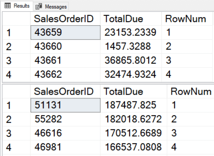
Since the first query is using the cluster key as the ORDER BY option, no sorting is necessary.

The second query has an expensive sort operation.

The ORDER BY in the OVER clause is not connected to the ORDER BY clause added to the overall query which could be quite different. Here is an example showing what happens if the two are different:
|
1 2 3 4 5 |
SELECT SalesOrderID, TotalDue, ROW_NUMBER() OVER(ORDER BY TotalDue DESC) AS RowNum FROM Sales.SalesOrderHeader ORDER BY SalesOrderID; |
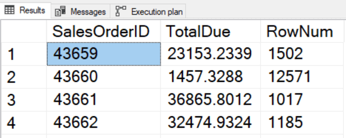
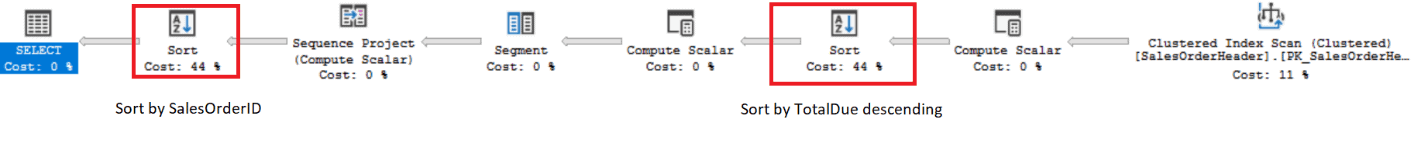
The clustered index key is SalesOrderID, but the rows must first be sorted by TotalDue in descending order and then back to SalesOrderID. Take a look at the execution plan:
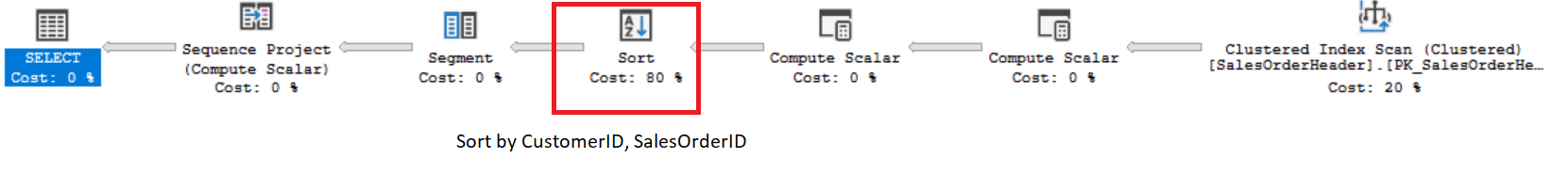
The PARTITION BY clause, supported but optional, for all T-SQL window functions also causes sorting. It’s similar to, but not exactly like, the GROUP BY clause for aggregate queries. This example starts the row numbers over for each customer.
|
1 2 3 4 5 6 |
SELECT CustomerID, SalesOrderID, TotalDue, ROW_NUMBER() OVER(PARTITION BY CustomerID ORDER BY SalesOrderID) AS RowNum FROM Sales.SalesOrderHeader; |
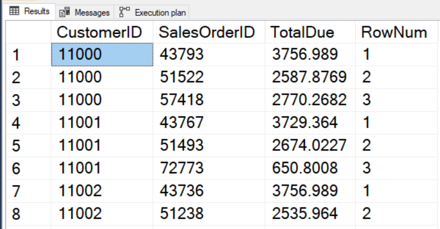
The execution plan shows just one sort operation, a combination of CustomerID and SalesOrderID.
The only way to overcome the performance impact of sorting is to create an index specifically for the OVER clause. In his book Microsoft SQL Server 2012 High-Performance T-SQL Using Window Functions, Itzik Ben-Gan recommends the POC index. POC stands for (P)ARTITION BY, (O)RDER BY, and (c)overing. He recommends adding any columns used for filtering before the PARTITION BY and ORDER BY columns in the key. Then add any additional columns needed to create a covering index as included columns. Just like anything else, you will need to test to see how such an index impacts your query and overall workload. Of course, you cannot add an index for every query that you write, but if the performance of a particular query that uses a window function is important, you can try out this advice.
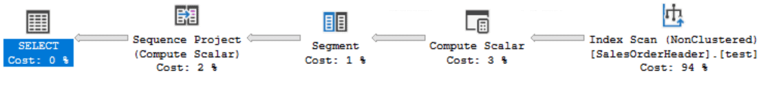
Here is an index that will improve the previous query:
|
1 2 3 |
CREATE NONCLUSTERED INDEX test ON Sales.SalesOrderHeader (CustomerID, SalesOrderID) INCLUDE (TotalDue); |
When you rerun the query, the sort operation is now gone from the execution plan:
Read Also: Closure tables for hierarchical queries
Framing
In my opinion, framing is the most difficult concept to understand when learning about T-SQL window functions. To learn more about the syntax see introduction to T-SQL window functions. Framing is required for the following:
- Window aggregates with the ORDER by, used for running totals or moving averages, for example
- FIRST_VALUE
- LAST_VALUE
Luckily, framing is not required most of the time, but unfortunately, it’s easy to skip the frame and use the default. The default frame is always RANGE BETWEEN UNBOUNDED PRECEDING AND CURRENT ROW. While you will get the correct results as long as the ORDER BY option consists of a unique column or set of columns, you will see a performance hit.
Here is an example comparing the default frame to the correct frame:
|
1 2 3 4 5 6 7 8 9 10 11 12 13 14 15 16 |
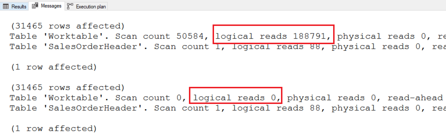
SET STATISTICS IO ON; GO SELECT CustomerID, SalesOrderID, TotalDue, SUM(TotalDue) OVER(PARTITION BY CustomerID ORDER BY SalesOrderID) AS RunningTotal FROM Sales.SalesOrderHeader; SELECT CustomerID, SalesOrderID, TotalDue, SUM(TotalDue) OVER(PARTITION BY CustomerID ORDER BY SalesOrderID ROWS BETWEEN UNBOUNDED PRECEDING AND CURRENT ROW) AS RunningTotal FROM Sales.SalesOrderHeader; |
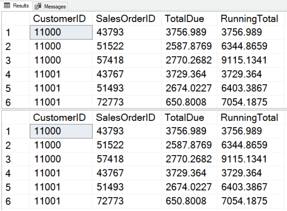
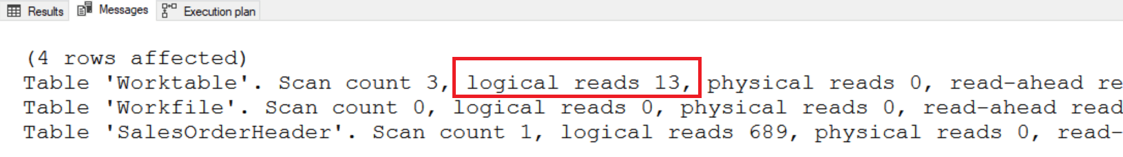
The results are the same, but the performance is very different. Unfortunately, the execution plan doesn’t tell you the truth in this case. It reports that each query took 50% of the resources:
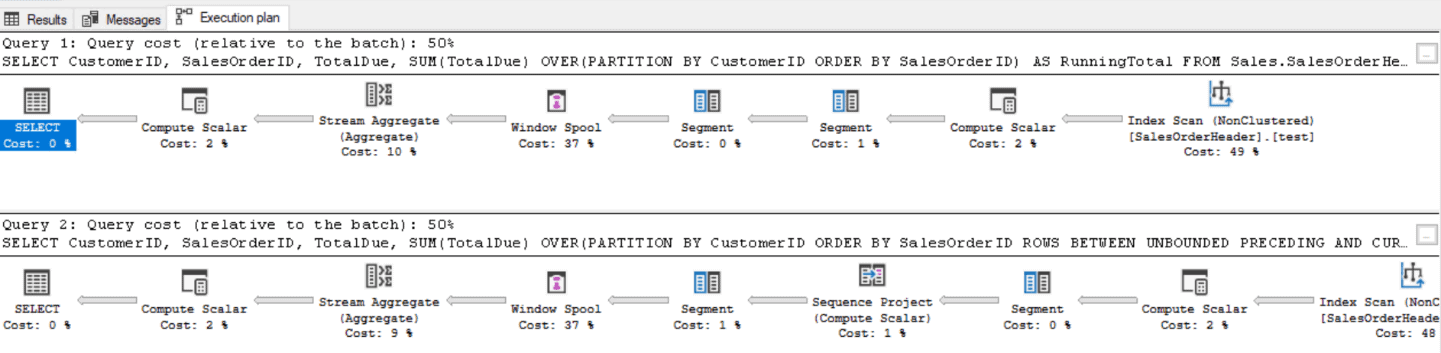
If you review the statistics IO values, you will see the difference:
Using the correct frame is even more important if your ORDER BY option is not unique or if you are using LAST_VALUE. In this example, the ORDER BY column is OrderDate, but some customers have placed more than one order on a given date. When not specifying the frame, or using RANGE, the function treats matching dates as part of the same window.
|
1 2 3 4 5 6 7 8 9 10 11 |
SELECT CustomerID, SalesOrderID, TotalDue, OrderDate, SUM(TotalDue) OVER(PARTITION BY CustomerID ORDER BY OrderDate) AS RunningTotal, SUM(TotalDue) OVER(PARTITION BY CustomerID ORDER BY OrderDate ROWS BETWEEN UNBOUNDED PRECEDING AND CURRENT ROW) AS CorrectRunningTotal FROM Sales.SalesOrderHeader WHERE CustomerID IN ('11433','11078','18758'); |
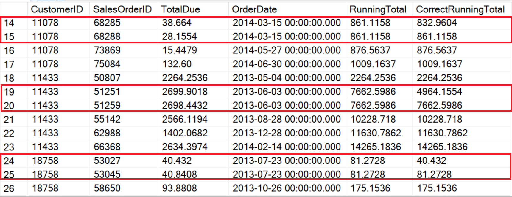
The reason for the discrepancy is that RANGE sees the data logically while ROWS sees it positionally. There are two solutions for this problem. One is to make sure that the ORDER BY option is unique. The other and more important option is to always specify the frame where it’s supported.
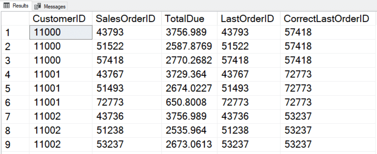
The other place that framing causes logical problems is with LAST_VALUE. LAST_VALUE returns an expression from the last row of the frame. Since the default frame (RANGE BETWEEN UNBOUNDED PRECEDING AND CURRENT ROW) only goes up to the current row, the last row of the frame is the row where the calculation is being performed. Here is an example:
|
1 2 3 4 5 6 7 8 9 10 11 |
SELECT CustomerID, SalesOrderID, TotalDue, LAST_VALUE(SalesOrderID) OVER(PARTITION BY CustomerID ORDER BY SalesOrderID) AS LastOrderID, LAST_VALUE(SalesOrderID) OVER(PARTITION BY CustomerID ORDER BY SalesOrderID ROWS BETWEEN CURRENT ROW AND UNBOUNDED FOLLOWING) AS CorrectLastOrderID FROM Sales.SalesOrderHeader ORDER BY CustomerID, SalesOrderID; |
Window Aggregates
One of the handiest feature of T-SQL window functions is the ability to add an aggregate expression to a non-aggregate query. Unfortunately, this can often perform poorly. To see the problem, you need to look at the statistics IO results where you will see a large number of logical reads. My advice when you need to return values at different granularities within the same query for a large number of rows is to use one of the older techniques, such as a common table expression (CTE), temp table, or even a variable. If it’s possible to pre-aggregate before using the window aggregate, that is another option. Here is an example that shows the difference between a window aggregate and another technique:
|
1 2 3 4 5 6 7 8 9 10 11 12 13 14 15 16 17 |
SELECT SalesOrderID, TotalDue, SUM(TotalDue) OVER() AS OverallTotal FROM Sales.SalesOrderHeader WHERE YEAR(OrderDate) =2013; DECLARE @OverallTotal MONEY; SELECT @OverallTotal = SUM(TotalDue) FROM Sales.SalesOrderHeader WHERE YEAR(OrderDate) = 2013; SELECT SalesOrderID, TotalDue, @OverallTotal AS OverallTotal FROM Sales.SalesOrderHeader AS SOH WHERE YEAR(OrderDate) = 2013; |
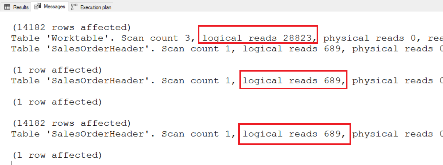
The first query only scans the table once, but it has 28,823 logical reads in a worktable. The second method scans the table twice, but it doesn’t need the worktable.
The next example uses a windows aggregate applied to an aggregate expression:
|
1 2 3 4 5 6 7 |
SELECT YEAR(OrderDate) AS OrderYear, SUM(TotalDue) AS YearTotal, SUM(TotalDue)/ SUM(SUM(TotalDue)) OVER() * 100 AS PercentOfSales FROM Sales.SalesOrderHeader GROUP BY YEAR(OrderDate) ORDER BY OrderYear; |
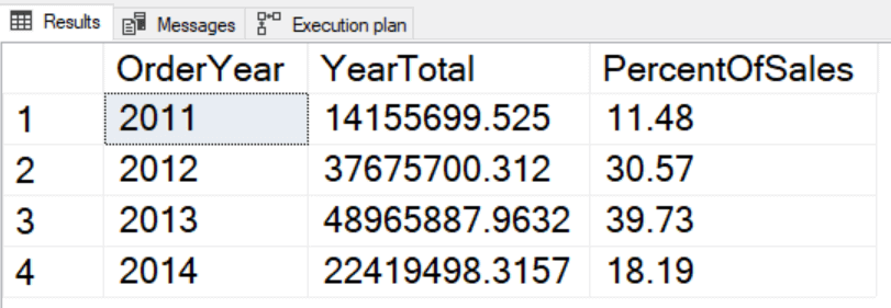
When using window functions in an aggregate query, the expression must follow the same rules as the SELECT and ORDER BY clauses. In this case, the window function is applied to SUM(TotalDue). It looks like a nested aggregate, but it’s really a window function applied to an aggregate expression.
Since the data has been aggregated before the window function was applied, the performance is good:
There is one more interesting thing to know about using window aggregates. If you use multiple expressions that use matching OVER clause definitions, you will not see an additional degradation in performance.
My advice is to use this functionality with caution. It’s quite handy but doesn’t scale that well.
Read also: Subqueries as alternatives to window functions
Performance Comparisons
The examples presented so far have used the small Sales.SalesOrderHeader table from AdventureWorks and reviewed the execution plans and logical reads. In real life, your customers will not care about the execution plan or the logical reads; they will care about how fast the queries run. To better see the difference in run times, I used Adam Machanic’s Thinking Big (Adventure) script with a twist.
The script creates a table called bigTransactionHistory containing over 30 million rows. After running Adam’s script, I created two more copies of his table, with 15 and 7.5 million rows respectively. I also turned on the Discard results after execution property in the Query Editor so that populating the grid did not affect the run times. I ran each test three times and cleared the buffer cache before each run.
Here is the script to create the extra tables for the test:
|
1 2 3 4 5 6 7 8 9 10 11 12 13 14 15 16 17 18 19 20 21 22 23 24 25 26 27 28 29 30 31 32 33 34 35 36 37 38 39 40 41 |
SELECT TOP(50) Percent * INTO mediumTransactionHistory FROM bigTransactionHistory; SELECT TOP(25) PERCENT * INTO smallTransactionHistory FROM bigTransactionHistory; GO ALTER TABLE mediumTransactionHistory ALTER COLUMN TransactionID INT NOT NULL; GO ALTER TABLE mediumTransactionHistory ADD CONSTRAINT pk_mediumTransactionHistory PRIMARY KEY (TransactionID); GO ALTER TABLE smallTransactionHistory ALTER COLUMN TransactionID INT NOT NULL; GO ALTER TABLE smallTransactionHistory ADD CONSTRAINT pk_smallTransactionHistory PRIMARY KEY (TransactionID); GO CREATE NONCLUSTERED INDEX IX_ProductId_TransactionDate ON mediumTransactionHistory ( ProductId, TransactionDate ) INCLUDE ( Quantity, ActualCost ); CREATE NONCLUSTERED INDEX IX_ProductId_TransactionDate ON smallTransactionHistory ( ProductId, TransactionDate ) INCLUDE ( Quantity, ActualCost ); |
I can’t say enough about how important it is to use the frame when it’s supported. To see the difference, I ran a test to calculate running totals using four methods:
- Cursor solution
- Correlated sub-query
- Window function with default frame
- Window function with ROWS
I ran the test on the three new tables. Here are the results in a chart format:
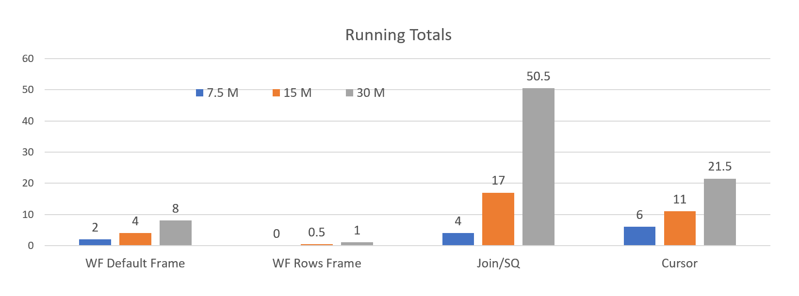
When running with the ROWS frame, the 7.5 million row table took less than a second to run on the system I was using when performing the test. The 30 million row table took about one minute to run.
Here is the query using the ROWS frame against the 30 million row table:
|
1 2 3 4 5 |
SELECT ProductID, SUM(ActualCost) OVER(PARTITION BY ProductID ORDER BY TransactionDate ROWS BETWEEN UNBOUNDED PRECEDING AND CURRENT ROW) AS RunningTotal FROM bigTransactionHistory; |
I also performed a test to see how window aggregates performed compared to traditional techniques. In this case, I used just the 30 million row table, but performed one, two, or three calculations using the same granularity and, therefore, same OVER clause. I compared the window aggregate performance to a CTE and to a correlated subquery.
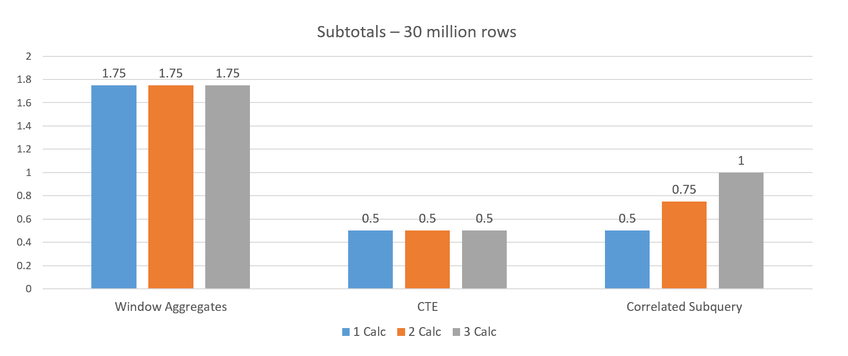
The window aggregate performed the worst, about 1.75 minutes in each case. The CTE performed the best when increasing the number of calculations since the table was just touched once for all three. The correlated subquery performed worse when increasing the number of calculations since each calculation had to run separately, and it touched the table a total of four times.
Here is the winning query:
|
1 |
WITH Calcs AS (<br> SELECT ProductID,<br> AVG(ActualCost) AS AvgCost, <br> MIN(ActualCost) AS MinCost,<br> MAX(ActualCost) AS MaxCost<br> FROM bigTransactionHistory<br> GROUP BY ProductID)<br>SELECT O.ProductID, <br> ActualCost,<br> AvgCost, <br> MinCost,<br> MaxCost <br>FROM bigTransactionHistory AS O <br>JOIN Calcs ON O.ProductID = Calcs.ProductID; |
Read also: Columnstore indexes for analytical queries
Conclusion
T-SQL window functions have been promoted as being great for performance. In my opinion, they make writing queries easier, but you need to understand them well to get good performance. Indexing can make a difference, but you can’t create an index for every query you write. Framing may not be easy to understand, but it is so important if you need to scale up to large tables.
Read also: Temporary tables for pre-aggregation
Fast, reliable and consistent SQL Server development…
FAQs: T-SQL Window Functions and Performance
1. How do you improve window function performance in SQL Server?
Create an index matching the PARTITION BY and ORDER BY columns in your OVER clause. For OVER(PARTITION BY CustomerID ORDER BY OrderDate), create an index on (CustomerID, OrderDate) with any SELECT columns as INCLUDE columns. This eliminates the sort operation – the most expensive part of window function execution.
2. What is NTILE in SQL and how does it work?
NTILE(n) divides an ordered result set into n approximately equal groups and assigns a group number (1 through n) to each row. NTILE(4) creates quartiles, NTILE(10) deciles. Requires ORDER BY in the OVER clause. Rows are distributed as evenly as possible; if not perfectly divisible, earlier groups get one extra row. Combine with PARTITION BY for groups within categories.
3. What is the difference between ROWS and RANGE framing in window functions?
ROWS defines the frame by physical row positions (ROWS BETWEEN 1 PRECEDING AND 1 FOLLOWING = exactly 3 rows). RANGE defines it by logical value ranges, including all ties. RANGE is SQL Server’s default and requires an on-disk spool, which is slower. Always specify ROWS explicitly for running totals and moving averages to avoid the RANGE performance penalty.
4. Can you use COUNT DISTINCT as a window function in SQL Server?
No. COUNT(DISTINCT) is not supported as a window function. Workaround: use a CTE with GROUP BY for the distinct count, then JOIN back. Or use DENSE_RANK to assign unique rankings and COUNT the results.
This document contains proprietary information and is protected by copyright law.
Copyright © 2026 Red Gate Software Limited. All rights reserved


Load comments