
I’ve spent the past six years traveling around the US telling database professionals about T-SQL Window Functions at SQL Saturdays and other events. I’m amazed at how few people have heard about these functions and even fewer who are using them. At the end of each presentation, one or more people come up to say that they wished they learned about these functions years earlier because they could have been beneficial for so many queries.
These functions have been promoted to improve performance over other, more traditional methods. I partially agree. They make many queries easier to write, and, sometimes, they improve performance.
Nothing to do with the Windows OS
These functions are part of the ANSI SQL 2003 Standards and, in the case of SQL Server, are T-SQL functions used to write queries. They have nothing to do with the Windows operating system or any API calls. Other database systems, such as Oracle, have also included these as part of their own SQL language.
Window (also, windowing or windowed) functions perform a calculation over a set of rows. I like to think of “looking through the window” at the rows that are being returned and having one last chance to perform a calculation. The window is defined by the OVER clause which determines if the rows are partitioned into smaller sets and if they are ordered. In fact, if you use a window function you will always use an OVER clause. The OVER clause is also part of the NEXT VALUE FOR syntax required for the sequence object, but, otherwise it’s used with window functions.
The OVER clause may contain a PARTITION BY option. This breaks the rows into smaller sets. You might think that this is the same as GROUP BY, but it’s not. When grouping, one row per unique group is returned. When using PARTITION BY, all of the detail rows are returned along with the calculations. If you have a window in your home that is divided into panes, each pane is a window. When thinking about window functions, the entire set of results is a partition, but when using PARTITION BY, each partition can also be considered a window. PARTITION BY is supported – and optional – for all windowing functions.
The OVER clause may also contain an ORDER BY option. This is independent of the ORDER BY clause of the query. Some of the functions require ORDER BY, and it’s not supported by the others. When the order of the rows is important when applying the calculation, the ORDER BY is required.
Window functions may be used only in the SELECT and ORDER BY clauses of a query. They are applied after any joining, filtering, or grouping.
Ranking Functions
The most commonly used window functions, ranking functions, have been available since 2005. That’s when Microsoft introduced ROW_NUMBER, RANK, DENSE_RANK, and NTILE. ROW_NUMBER is used very frequently, to add unique row numbers to a partition or to the entire result set. Adding a row number, or one of the other ranking functions, is not usually the goal, but it is a step along the way to the solution.
ORDER BY is required in the OVER clause when using ROW_NUMBER and the other functions in this group. This tells the database engine the order in which the numbers should be applied. If the values of the columns or expressions used in the ORDER BY are not unique, then RANK and DENSE_RANK will deal with the ties, while ROW_NUMBER doesn’t care about ties. NTILE is used to divide the rows into buckets based on the ORDER BY.
One benefit of ROW_NUMBER is the ability to turn non-unique rows into unique rows. This could be used to eliminate duplicate rows, for example.
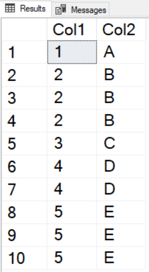
To show how this works, start with a temp table containing duplicate rows. The first step is to create the table and populate it.
|
1 2 3 4 5 6 |
CREATE TABLE #Duplicates(Col1 INT, Col2 CHAR(1)); INSERT INTO #Duplicates(Col1, Col2) VALUES(1,'A'),(2,'B'),(2,'B'),(2,'B'), (3,'C'),(4,'D'),(4,'D'),(5,'E'), (5,'E'),(5,'E'); SELECT * FROM #Duplicates; |
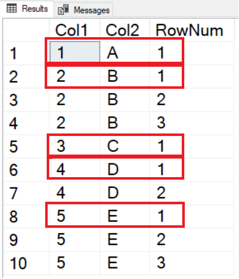
Adding ROW_NUMBER and partitioning by each column will restart the row numbers for each unique set of rows. You can identify the unique rows by finding those with a row number equal to one.
|
1 2 3 |
SELECT Col1, Col2, ROW_NUMBER() OVER(PARTITION BY Col1, Col2 ORDER BY Col1) AS RowNum FROM #Duplicates; |
Now, all you have to do is to delete any rows that have a row number greater than one. The problem is that you cannot add window functions to the WHERE clause.
|
1 2 |
DELETE #Duplicates WHERE ROW_NUMBER() OVER(PARTITION BY Col1, Col2 ORDER BY Col1) <> 1; |
You’ll see this error message:

The way around this problem is to separate the logic using a common table expression (CTE). You can then delete the rows right from the CTE.
|
1 2 3 4 5 6 7 |
WITH Dupes AS ( SELECT Col1, Col2, ROW_NUMBER() OVER(PARTITION BY Col1, Col2 ORDER BY Col1) AS RowNum FROM #Duplicates) DELETE Dupes WHERE RowNum <> 1; SELECT * FROM #Duplicates; |
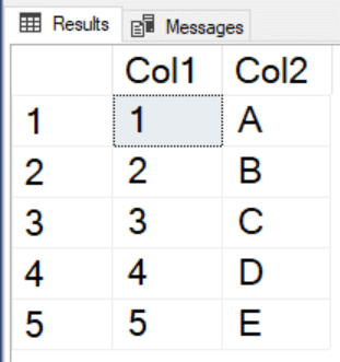
Success! The extra rows were deleted, and a unique set of rows remains.
To see the difference between ROW_NUMBER, RANK, and DENSE_RANK, run this query:
|
1 2 3 4 5 6 7 8 |
USE Adventureworks2017; --Or whichever version you have GO SELECT SalesOrderID, OrderDate, CustomerID, ROW_NUMBER() OVER(ORDER BY OrderDate) As RowNum, RANK() OVER(ORDER BY OrderDate) As Rnk, DENSE_RANK() OVER(ORDER BY OrderDate) As DenseRnk FROM Sales.SalesOrderHeader WHERE CustomerID = 11330; |
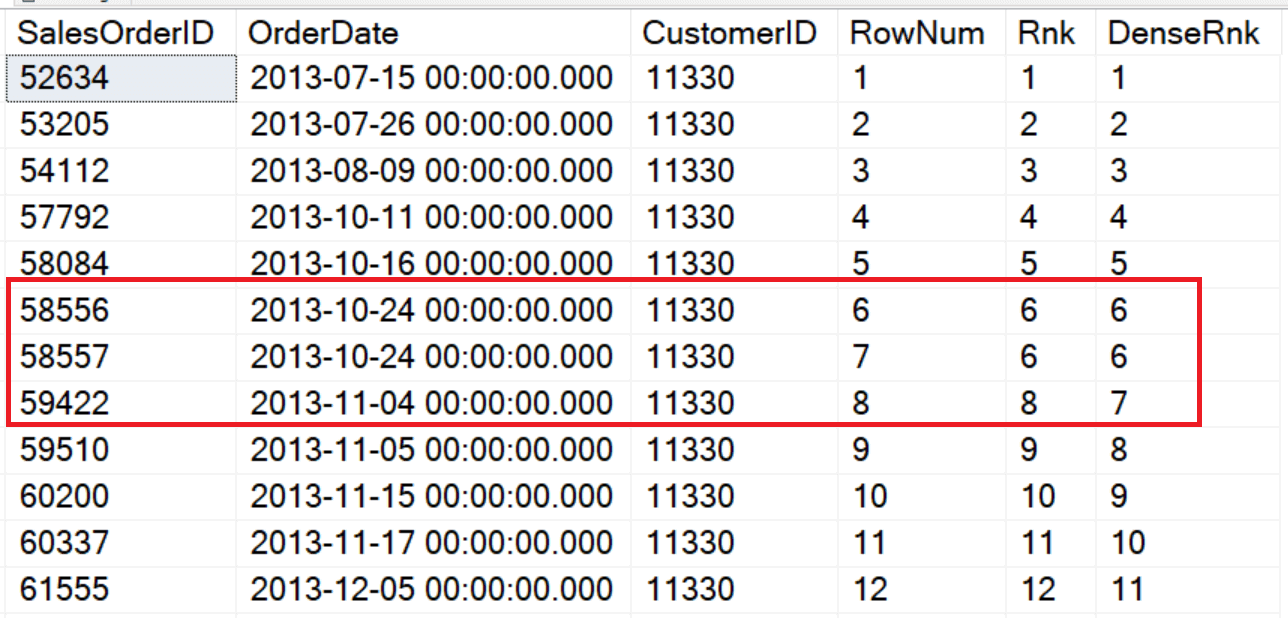
The ORDER BY for each OVER clause is OrderDate which is not unique. This customer placed two orders on 2013-10-24. ROW_NUMBER just continued assigning numbers and didn’t do anything different even though there is a duplicate date. RANK assigned 6 to both rows and then caught up to ROW_NUMBER with an 8 on the next row. DENSE_RANK also assigned 6 to the two rows but assigned 7 to the following row.
Two explain the difference, think of ROW_NUMBER as positional. RANK is both positional and logical. Those two rows are ranked logically the same, but the next row is ranked by the position in the set. DENSE_RANK ranks them logically. Order 2013-11-04 is the 7th unique date.
The final function in this group is called NTILE. It assigns bucket numbers to the rows instead of row numbers or ranks. Here is an example:
|
1 2 3 4 5 6 7 8 |
SELECT SP.FirstName, SP.LastName, SUM(SOH.TotalDue) AS TotalSales, NTILE(4) OVER(ORDER BY SUM(SOH.TotalDue)) * 1000 AS Bonus FROM [Sales].[vSalesPerson] SP JOIN Sales.SalesOrderHeader SOH ON SP.BusinessEntityID = SOH.SalesPersonID WHERE SOH.OrderDate >= '2012-01-01' AND SOH.OrderDate < '2013-01-01' GROUP BY FirstName, LastName; |
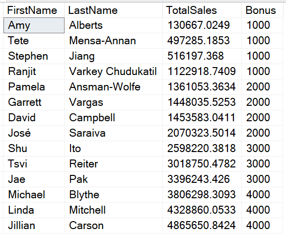
NTILE has a parameter, in this case 4, which is the number of buckets you want to see in the results. The ORDER BY is applied to the sum of the sales. The rows with the lowest 25% are assigned 1, the rows with the highest 25% are assigned 4. Finally, the results of NTILE are multiplied by 1000 to come up with the bonus amount. Since 14 cannot be evenly divided by 4, an extra row goes into each of the first two buckets.
Window Aggregates
Window aggregates were also introduced with SQL Server 2005. These make writing some tricky queries easy but will often perform worse than older techniques. They allow you to add your favourite aggregate function to a non-aggregate query. Say, for example you would like to display all the customer orders along with the subtotal for each customer. By adding a SUM using the OVER clause, you can accomplish this very easily:
|
1 2 3 |
SELECT CustomerID, OrderDate, SalesOrderID, TotalDue, SUM(TotalDue) OVER(PARTITION BY CustomerID) AS SubTotal FROM Sales.SalesOrderHeader; |
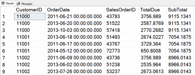
By adding the PARTITION BY, a subtotal is calculated for each customer. Any aggregate function can be used, and ORDER BY in the OVER clause is not supported.
Window Aggregate Enhancements in 2012
Beginning with 2012, you can add an ORDER BY to the OVER clause to window aggregates to produce running totals and moving averages, for example. At the same time, Microsoft introduced the concept of framing. Adding a PARTITION BY is like dividing a window into panes. Adding framing is like creating a stained-glass window. Each row has an individual window where the expression will be applied.
With this enhancement, you can create running totals even without adding the framing syntax. Here is an example that returns a running total by customer:
|
1 2 3 4 |
SELECT CustomerID, OrderDate, SalesOrderID, TotalDue, SUM(TotalDue) OVER(PARTITION BY CustomerID ORDER BY SalesOrderID) AS RunningTotal FROM Sales.SalesOrderHeader; |
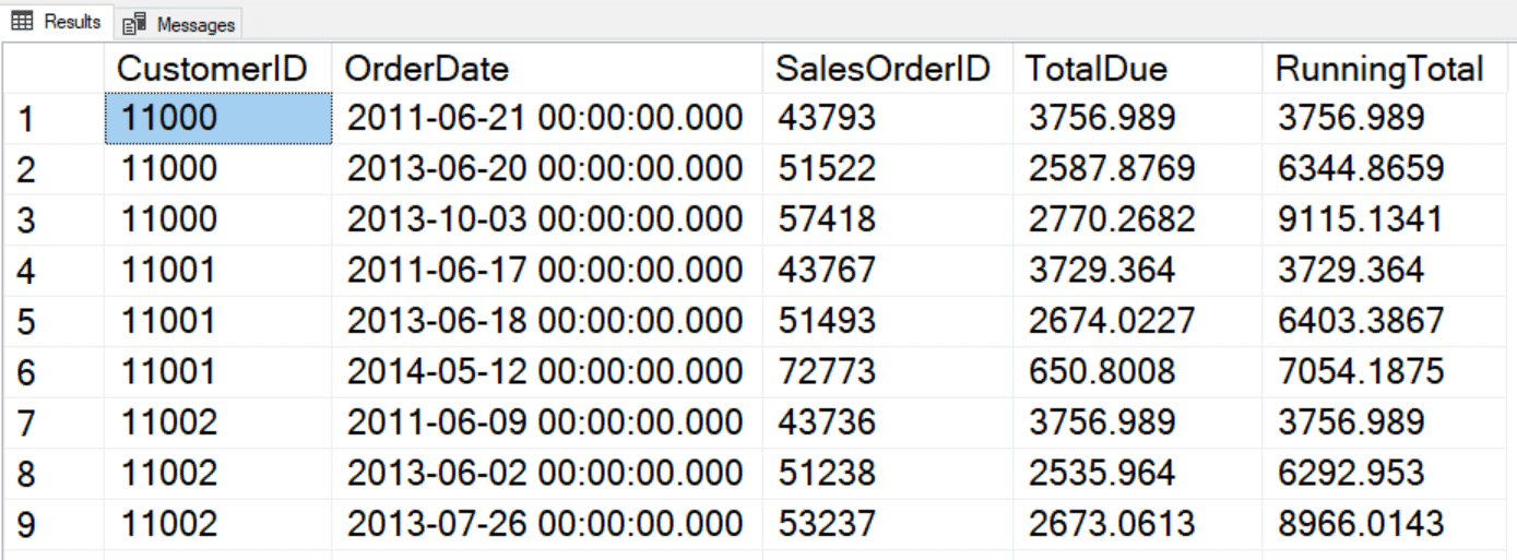
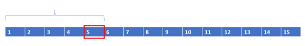
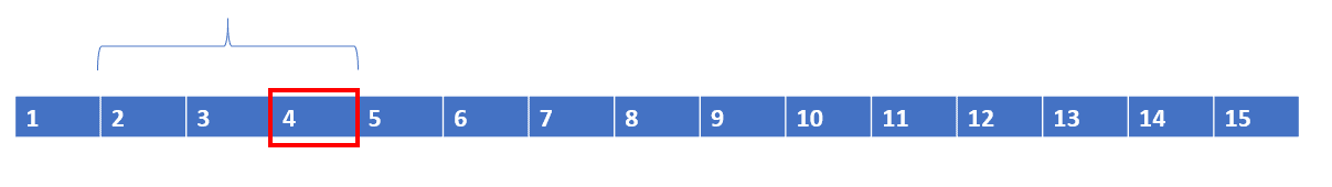
The default frame, which is used if a frame is not specified, is RANGE BETWEEN UNBOUNDED PRECEDING AND CURRENT ROW. Unfortunately, this will not perform as well as if you specify this frame instead: ROWS BETWEEN UNBOUNDED PRECEDING AND CURRENT ROW. The difference is the word ROWS. RANGE is only partially implemented at this time, and it’s meant for working with periods of time, while ROWS is positional. The frame, ROWS BETWEEN UNBOUNDED PRECEDING AND CURRENT ROW, means that the window consists of the first row of the partition and all the rows up to the current row. Each calculation is done over a different set of rows. For example, when performing the calculation for row 4, the rows 1 to 4 are used.
When performing the calculation for row 5, the rows are 1 to 5. The window grows larger as you move from one row to the next.
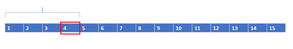
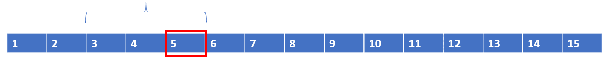
You can also use the syntax ROWS BETWEEN N PRECEEDING AND CURRENT ROW or ROWS BETWEEN CURRENT ROW AND N FOLLOWING. This could be useful for calculating a three-month moving average, for example. The following figure represents ROWS BETWEEN 2 PRECEDING AND CURRENT ROW.
When 5 is the current row, the window moves; it doesn’t change size.
Here is the list of terms you need to know when writing the framing option:
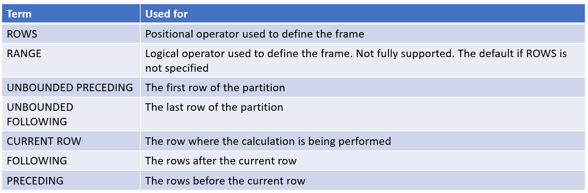
I admit that this syntax is a bit confusing but using SQL Prompt helps makes writing the framing option easier!
Offset Functions
Also included with the release of SQL Server 2012 are four functions that allow you to include values from other rows – without doing a self-join. Microsoft calls these ‘analytic functions’, but I always refer to them as ‘offset functions’ when presenting on this topic. Two of the functions allow you to pull columns or expressions from a row before (LAG) or after (LEAD) the current row. The other two functions allow you to return values from the first row of the partition (FIRST_VALUE) or last row of the partition (LAST_VALUE). FIRST_VALUE and LAST_VALUE also require framing, so be sure to include the frame when using these functions. All four of the functions require the ORDER BY option of the OVER clause. That makes sense, because the database engine must know the order of the rows to figure out which row contains the value to return.
Some people have a favourite band; some people have a favourite movie. I have a favourite function – LAG. It’s easy to use (no frame!) and performs great. Here is an example:
|
1 2 3 4 5 |
SELECT CustomerID, OrderDate, SalesOrderID, LAG(SalesOrderID) OVER(PARTITION BY CustomerID ORDER BY SalesOrderID ) AS PrevOrder FROM Sales.SalesOrderHeader ORDER BY CustomerID; |
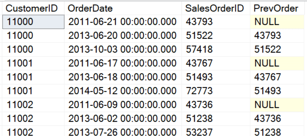
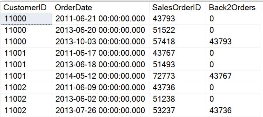
LAG and LEAD require an argument – the column or expression you want to return. By default, LAG returns the value from the previous row, and LEAD returns the value from the following row. You can modify that by supplying a value for the OFFSET parameter, which is 1 by default. Notice that the first row of the partition returns NULL. If you wish to override the NULLs, you can supply a DEFAULT value. Here is a similar query that goes back two rows and has a default value:
|
1 2 3 4 |
SELECT CustomerID, OrderDate, SalesOrderID, LAG(SalesOrderID,2,0) OVER(PARTITION BY CustomerID ORDER BY SalesOrderID) AS Back2Orders FROM Sales.SalesOrderHeader; |
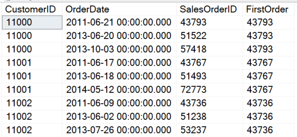
FIRST_VALUE and LAST_VALUE can be used to find a value from the very first row or very last row of the partition. Be sure to specify the frame, not only for performance reasons, but because the default frame doesn’t work as you would expect with LAST_VALUE. The default frame, RANGE BETWEEN UNBOUNDED PRECEDING AND CURRENT ROW, only goes up to the current row. The last row of the partition is not included. To get the expected results, be sure to specify ROWS BETWEEN CURRENT ROW AND UNBOUNDED FOLLOWING when using LAST_VALUE. Here is an example using FIRST_VALUE:
|
1 2 3 4 5 |
SELECT CustomerID, OrderDate, SalesOrderID, FIRST_VALUE(SalesOrderID) OVER(PARTITION BY CustomerID ORDER BY SalesOrderID ROWS BETWEEN UNBOUNDED PRECEDING AND CURRENT ROW) AS FirstOrder FROM Sales.SalesOrderHeader; |
Statistical Functions
Microsoft groups these four functions – PERCENT_RANK, CUME_DIST, PERCENTILE_DISC, PERCENTILE_CONT – along with the offset functions calling all eight the analytic functions. Since I like to distinguish these from the offset functions, I call these statistical.
PERCENT_RANK and CUME_DIST provide a ranking for each row over a partition. They differ slightly. PERCENT_RANK returns the percentage of rows that rank lower than the current row. “My score is higher than 90% of the scores.” CUME_DIST, or cumulative distribution, returns the exact rank. “My score is at 90% of the scores.” Here is an example using the average high temperature in St. Louis for each month. Note that the ranks were determined by the Fahrenheit temperature.
|
1 2 3 4 5 6 7 8 9 10 11 |
CREATE TABLE #MonthlyTempsStl(MName varchar(15), AvgHighTempF INT, AvgHighTempC INT) INSERT INTO #MonthlyTempsStl(MName, AvgHighTempF, AvgHighTempC) VALUES('Jan',40,4),('Feb',45, 7),('Mar',56, 13),('Apr',67, 20), ('May',76,25),('Jun',85,30),('Jul',89,32),('Aug',88,31), ('Sep',80,27),('Oct',69,20),('Nov',56,13),('Dec',43,6); SELECT MName, AvgHighTempF,AvgHighTempC, RANK() OVER(ORDER BY AvgHighTempF) AS Rank, PERCENT_RANK() OVER(ORDER BY AvgHighTempF) AS PercentRank, CUME_DIST() OVER(ORDER BY AvgHighTempF) AS CumeDist FROM #MonthlyTempsStl; |
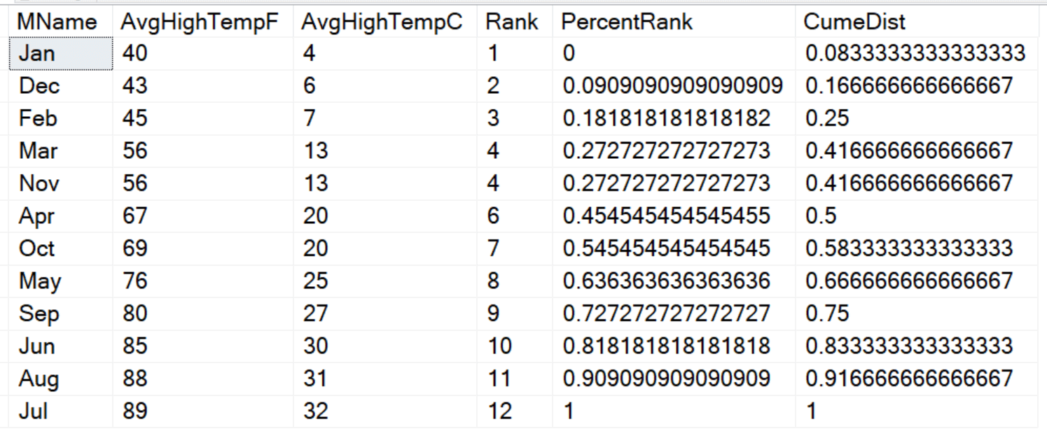
The ranks are not determined by the relative values, but by the positions of the rows. Notice that March and November have the same average high temp, so they were ranked the same.
You may be wondering how to calculate PERCENT_RANK and CUME_DIST. Here are the formulas:
|
1 2 |
PERCENT_RANK = (Rank -1)/(Row count -1) CUME_DIST = (Rank)/(Row count) |
PERCENTILE_DISC and PERCENTILE_CONT work in the opposite way. Given a percent rank, find the value at that rank. They differ in that PERCENTILE_DISC will return a value that exists in the set while PERCENTILE_CONT will calculate an exact value if none of the values in the set falls precisely at that rank. You can use PERCENTILE_CONT to calculate a median by supplying 0.5 as the percent rank. For example, which temperature ranks at 50% in St. Louis?
|
1 2 3 4 5 6 7 |
SELECT MName, AvgHighTempF,AvgHighTempC, RANK() OVER(ORDER BY AvgHighTempF) AS Rank, PERCENTILE_CONT(0.5) WITHIN GROUP(ORDER BY AvgHighTempF) OVER() AS PercentileCont, PERCENTILE_DISC(0.5) WITHIN GROUP(ORDER BY AvgHighTempF) OVER() AS PercentileDisc FROM #MonthlyTempsStl; |
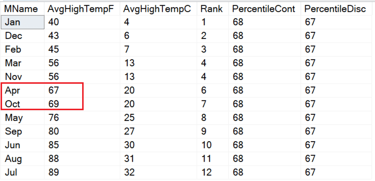
The PERCENTILE_CONT function takes the average of the two values closest to the middle, 67 and 69, and averages them. PERCENTILE_DISC returns an exact value, 67. Also notice that these two functions have an extra clause not seen in the other functions, WITHIN GROUP, that contains the ORDER BY instead of within the OVER clause.
Summary
This article is a very quick overview of T-SQL window functions. Two types of functions were released with SQL Server 2005, the ranking functions and window aggregates. With 2012, you have enhanced window aggregate with framing and the analytic functions. I like to separate the analytic functions into two groups, the offset and statistical functions. Window functions make many queries easier to write, and I believe that is the main benefit. In some cases, the queries will perform better, too, but that is a discussion for another day.
I hope this article has inspired you to learn more about these fantastic functions!
This document contains proprietary information and is protected by copyright law.
Copyright © 2026 Red Gate Software Limited. All rights reserved


Load comments