Contents

There is no statistics object at all

If there’s no statistics, the optimizer will have to guess row-counts rather than estimate them, and believe me: this is not what you want!

There are several ways of finding out from both the estimated and actual execution plans whether the optimizer comes across missing statistics. In this case you’ll see warnings in the plan. The there will be an exclamation mark in the graphical execution plan and a warning in the extended operator information, just like the one in Picture 1. You won’t see this warning for table variables, so watch out for table scans on table variables and their row-count estimations.

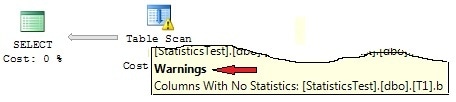
Picture 1: Missing statistics warning

If you want to have a look at execution plans for preceding queries, you may request these plans by the use of the sys.dm_exec_cached_plans DMV.

SQL Server Profiler offers another option. If you include the event Errors and Warnings/Missing Column Statistics in your profile, you’ll observe a log entry whenever the optimizer detects a missing statistics. Be aware however that this event will not be fired if AUTO CREATE STATISTICS is enabled for the database or table.

There are several circumstances under which you’ll experience missing statistics.

AUTO CREATE STATISTICS is OFF

Problem:

If you’ve set the option AUTO CREATE STATISTICS OFF and overlooked the task of creating statistics manually, the optimizer will suffer from missing statistics.

Solution:

Rely instead on the automatic creation of statistics by setting AUTO CREATE STATISTICS to ON.

Table variables

Problem:

For table variables, statistics will never be maintained. Keep that in mind: no statistics for table variables! When selecting from table variables, the estimated row-count is always 1, unless a predicate that evaluates to false, and doesn’t have any relationship to the table variable, is applied (such as WHERE 1=0), in which case the estimated row-count evaluates to 0.

Solution:

Don’t count on using table variables for temp tables if they are likely to contain more than a few rows. As a rule of thumb, use temporary tables (tables with a “#” as their name’s first character), rather than table variables, for temp tables with more than 100 rows.

XML and spatial data

Problem:

SQL Server does not maintain statistics for XML and spatial data types. That’s just a fact, not a problem. So, don’t try to find statistics for these columns, as they’re simply not there.

Solution:

If you experience performance problems with queries that have to search through XML data, or filter spatial columns e.g., XML or spatial indexes may help. But that’s another story and beyond the scope of this article.

Remote queries

Problem:

Suppose that you query a table from an Oracle database via a linked server connection and join this table to some local database tables. It’s perfectly understandable that SQL Server has no idea of any row-counts from that remote table, since it is residing in an Oracle database. This can occur, if you use OPENROWSET or OPENQUERY for remote data access.

But you may also face this issue out of the blue, when working with DMVs. A certain number of SQL Server’s DMVs are no more than a shell for querying data from internal tables. You may see a Remote Scan operator for SQL Server 2005 or a Table Valued Function operator for SQL Server 2008 in this case. Those operators have tied default cardinality estimations. (Depending on the server version and the operator, these are 1, 1000, or 10000.)

Have a look at the following query:

Here’s what BOL states:

“Returns a single row that displays the state information of the transaction in the current session.”

But look at the execution plan in Picture 2. No estimated row-count of 1 there. Apparently the optimizer does not take BOL content into account when generating the plan. You see the internal table DM_TRAN_CURRENT_TRANSACTION that is called by invoking OPENROWSET and an estimated row-count of 1000, which is far from reality.

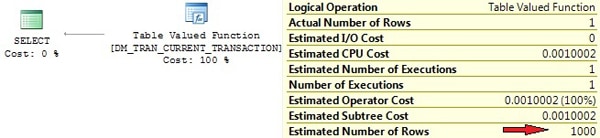
Picture 2: Row-count estimation for TVF

Solution:

If possible, give the optimizer some support by specifying the row-count through the TOP(n) clause. This will only be effective if n is less than the Estimated Number of Rows, 1000 in our example. So, if you have a guess of how many rows your Oracle query is about to return, just add TOP(n) to your OPENQUERY statement. This will help for better cardinality estimations and be useful if you utilize the OPENROWSET result for further joining or filtering. But be sure that this practice is somewhat dangerous. If you specify a value too low for n, your result set will lose rows, which would be a disaster.

With our example using sys.dm_tran_current_transaction , you would do better by rewriting the query like this:

Normally this won’t be necessary, because the simple SELECT, if used stand-alone, is quick enough. However, if you process the query result further by, perhaps, using it in joins, then the TOP 1 is useful.

If you find that you are using the OPENQUERY results in more complex queries for joining or filtering operations, then it is wise to import the OPENQUERY result into a local table first. Statistics and indexes can be properly maintained for this local table, so the optimizer then has enough information for realistic estimations of row-counts.

The database is read only

Problem:

If your database is set to read-only, the optimizer can’t add missing statistics even with AUTO CREATE STATISTICS enabled, because changes to read only databases are generally prevented.

Watch out for the fact that there is also a special kind of read only database. Yes, I’m talking about a snapshot! If the optimizer is missing the statistics for database snapshots, these can’t be created automatically. This is likely to happen if snapshots are being used for reporting applications. I often read suggestions to create snapshots for reporting purposes so as to avoid running those long running and resource-intensive reporting queries on the underlying OLPT systems. That may be fine up to a point, but Reporting queries are highly unpredictable and usually differ from normal OLTP queries. Therefore, there’s a chance that your reporting queries will suffer from missing statistics or, even worse, missing indexes.

Solution:

If you set your database to read-only, you’ll have to create your statistics manually before you do so.

Perfect statistics exist, but can’t be used properly

There is always a possibility that the optimizer cannot use statistics even if they are in place and up-to-date. This can be caused by poor TSQL code such as you’ll see in this section.

Utilization of local variables in TSQL scripts

Problem:

Let’s again have a look at this query form our introductory example:

Picture 5 of the first part shows the actual execution plan, which reveals a large discrepancy between the actual and estimated row-count. But what’s the reason for this difference?

If you’re familiar with the different steps of query execution, you’ll realize the answer to this. Before a query is executed, a query plan has to be generated, and right at the time of the compilation of the query, SQL Server does not know the value of variable @x. Yes of course, in our case it’d be easy to determine the value of @x, but there may be more complicated expressions that prevent the calculation of @x’s value at compile time In this case, the optimizer has no knowledge of the actual value of @x and is therefore unable to do a reasonable estimation of cardinality from the histogram.

But wait! At least there’s a statistics for column c1, so if the optimizer can’t browse the histogram, it may probably fall back to other, more general quantities. That’s exactly what happens here.

In case the optimizer can’t take advantage of a statistic’s histogram, the estimations of cardinality are determined by examining the average density, the total number of rows in the table, and possibly also the predicate’s operator(s). If you look at the example from the first part, you’ll see that we inserted 100001 rows into our test table, where column c1 had a value of 2000 for only one row and a value of 1000 for the remaining 100000 rows. You can inspect the average density of the statistics by executing DBCC SHOW_STATISTICS, but remember that this value calculates to 1/distinct number of values, which evaluates to 1/2=0.5 in our case. Hence, the optimizer calculates the average number of rows per distinct value of c1 to 100001 rows * 0.5 = 50000.5 rows. With this value at hand, the predicate’s operator comes into play, which is “=” in our example. For the exact comparison, the optimizer assumes that the average number of rows for one value of c1 will be returned, thus the expected row-count is 50000.5 (again, see Picture 5 of part one).

Other comparison operators lead to different estimates of selectivity, where the average density may or may not be considered. If ‘greater’ or ‘less than’ operators are applied, then it’s just assumed that 30% of all table rows will be returned. You can easily verify this by playing around with our little test script.

Solution(s):

If possible, avoid the using local variables in TSQL scripts. As this may not always be practicable, there are also other options available.

First, you may consider introducing stored procedures. These are perfectly designed for working with parameters by using a technique that’s called parameter sniffing. When a procedure is called for the first time, the optimizer will figure out any provided parameters and adjust the generated plan (and cardinality estimations, of course) according to these parameters. Although you might face other problems with this approach (see below), it is a perfect solution in our case.

If we embed our query into a stored procedure like this:

And then just execute this procedure by invoking:

The execution plan will expose an Index Seek, and thus look as it should. That’s because the optimizer knows it has to generate the plan for a value of @x=2000.

Picture 3 reveals the plan. Compare this to the original plan presented in Picture 5 of part one.

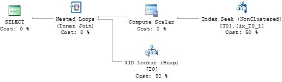
Picture 3: Execution plan of stored procedure

Secondly, you may consider solving the issue by the use of dynamic SQL. Ok, just to clarify this: No, no, no, I do not suggest using dynamic SQL in general and extensively. By no means would that be appropriate! Dynamic SQL has very bad side effects, such as possible Plan cache pollution, vulnerability to SQL injection attacks, and possibly increased CPU- and memory utilization. But look at this:

The execution plan is flawless now (same as in Picture 3), since it is created during the execution of the EXEC command, and the provided command string is passed as parameter to this command. In reality, you’d have to balance the consequences before deciding to use dynamic SQL. But you can see that, if carefully chosen and selectively applied, dynamic SQL is not bad in all cases. Altogether it’s very simple: just be aware of what you do!

More often than not the extended stored procedure sp_executesql will help you using dynamic SQL, while also excluding some of the dynamic SQL drawbacks at the same time.

Here’s our example again, this time re-written for sp_executesql:

Once more the execution plan looks like the one presented in Picture 3.

Providing expressions in predicates

Problem:

Using expressions in predicates may also prevent the optimizer from using the histogram. Look at the following example:

The execution plan is shown in Picture 4.

Picture 4: Bad cardinality estimation because of expression in predicate

So, although a statistics for columns c1 exists, the optimizer has no idea of how to apply this statistics to the expression POWER(c1,1) and therefore has to guess the row-count here. This is very similar to the problem of the missing statistics we’ve mentioned already, because there’s simply no statistics for the expression POWER(c1,1). In terms of the optimizer, POWER(c1,1) is called a non-foldable expression. Please refer to this article for more information.

Solution(s):

If possible, re-write your SQL Code so that comparisons are only done with “pure” columns. So e.g. instead of specifying

You would do better to write:

Fortunately the optimizer is quite smart when evaluating expressions and in some cases will do the re-write internally (again see here for some more information about this).

If re-writing your query is not possible, I suggest you ask a colleague for assistance. If it’s still not feasible, you may take calculated columns into account. Calculated columns will work out fine, since statistics are also maintained for calculated columns. Furthermore you may also create indexes for calculated columns, which you can’t do for expressions.

Parameterization issues

Problem:

If you use parameterized queries, such as the stored procedure in a previous example, you might face another problem. You’ll remember that the query plan is actually generated on the first call of the procedure, not the CREATE PROCEDURE statement. That’s the way, parameter sniffing works. The plan will be generated by utilizing row-count estimations for the provided parameter values that were provided at the first call. The problem here is quite obvious. What, if the first call is done with uncharacteristic parameter values? Cardinality estimations will use these values and the created execution plan then goes into the plan cache. The plan will have a poor estimation of row-counts, so subsequent reuse of the plan with more usual parameter values are likely to suffer poor performance.

Have a look at our stored procedure call:

If this is the first call of the procedure, the plan is generated for the filter WHERE c1=2000. Since there’s only one estimated row for c1=2000, an Index Seek is performed. If we’d call the procedure a second time like this:

The cached plan is re-used and again an Index Seek is performed. This is a very bad choice, because the query will now return 100000 rows. There is a big difference between the estimated and actual row-count! A Table Scan had been much more efficient here.

There’s another issue with parameterization that is very similar to the problem of using local variables in TSQL scripts that we’ve already written about. Consider this stored procedure:

Modifying the value of @x is not ideal. The parameter sniffing technique will not trace any modifications of @x, so the execution plan is adjusted to the provided value of @x only, not the actual value that is used inside the query. If you call the above stored procedure like this:

Then, the plan actually gets optimized for the filter WHERE c1=1000 and not WHERE c1=2000!

You really fool the optimizer by this practice, and unsatisfactory estimations of cardinality are highly likely to happen.

Solution:

If you are having problems that are caused by parameter sniffing, you can consider using query plan hints, such as OPTIMIZE FOR, or WITH RECOMPILE. This topic is outside the scope of this article, however.

Try not to modify parameter values within stored procedures. Doing so will outfox parameter sniffing. If you have to change parameter values for further processing, you might consider splitting the stored procedure into several smaller stored procedures. Introduce stored procedures in the sense of sub-routines. Modify any parameter values in the frame procedure and call your sub-routine procedure by using the changed value. As for every stored procedure, a separate plan is generated: This practice will circumvent the issue.

Statistics is too imprecise

Generally we have to accept a certain amount of uncertainty with distribution statistics. After all, statistics perform some data reduction, and information losses are inevitable. But if the information that we lose is crucial for the optimizer to make a proper estimate of cardinality, we must look for some other solution. How can statistics objects become just too imprecise to be useful?

Insufficient sample size

Problem:

Imagine a table with some million rows. Whenever SQL Server automatically creates or updates statistics for one of the columns of this table, it won’t take all of the table’s rows into account. To prevent exhaustive use of resources, like CPU and IO, usually only some sample rows are processed for the maintenance of statistics. This could lead to a histogram that poorly represents the overall distribution of data. If the optimizer estimates the cardinality, it may not be able to find enough information to generate an efficient query plan.

Solution:

The general solution is very simple. You’ll have to interfere in the automatic update or creation of statistics by manual updates or generation of statistics. Remember that you can specify the sample size or even perform a full scan when invoking CREATE STATISTICS or UPDATE STATISTICS.

Remember that an index rebuild will always force the production of statistics that are created with a full scan. Be aware though that an index rebuild has no effect on column statistics but only regards index-related statistics.

Statistics’ granularity is too broad

Problem:

Let’s come back to our table with multi-million rows again. Although the maximum size of the histogram is always limited to 200 entries, we know that we only have 200 clues for row-count estimations of a, let’s say a 4 million rows table. That’s an average of 4000000 rows/200 steps = 20000 rows per histogram step. If the column’s values were equally shared across all rows this won’t be a problem, but what if they aren’t? The statistics will probably be too coarse-grained and lead to inaccurate estimations of cardinality.

Solution:

Apparently it would be helpful to increase the histogram size, but we can’t do that can we? No, there’s no way of enlarging the size of a histogram to contain more than 200 entries. But if we can’t include more rows into one histogram, how about simply using more than one histogram? Of course we can achieve that by introducing filtered statistics. Since the histogram is always tied to a single statistics, we can have multiple histograms for the same column when using filtered statistics.

You will have to create these filtered statistics manually, and you’ll have to be aware of the consequences that I’ll explain a bit later.

Let’s just return to a previous example and imagine that we have a table containing 90% of historical data (that never get changed) and only 10% of active data. Gladly we decide on having two filtered statistics, and separate these two statistics objects by applying a filter condition to some date column. (You might prefer two filtered indexes but, for this illustration, it doesn’t matter whether it’s filtered indexes or statistics.) Additionally, we can disable automatic updates for the statistics that represent only historical data (the 90% part): This is because it is only our active part, the 10%-part, for which the statistics need to be regularly refreshed.

At this point we hit a problem: With CREATE AUTO STATISTICS set to ON, the optimizer will always add an unfiltered statistics object as well, even if filtered statistics for the same column already exist. This automatically-added statistics will also have the ‘automatic update’ option enabled. Therefore, although it may seem that the two filtered statistics are the only ones in place, one for the historical, and another one for the active part, you’ll end up with a total of three statistics, since another (unfiltered) one has been automatically added. Not only do we now have the superfluous unfiltered statistics but there will also be pointless automatic updates to it. Of course we could disable the automatic creation of statistics for the entire table, but this would put the onus on us for creating all appropriate statistics. I don’t like this idea very much. If there’s an automatic option, why not rely on it whenever possible.

I think the best way to overcome this issue is to create the unfiltered statistics manually by specifying the NORECOMPUTE option. This will prevent the optimizer from adding this statistics object and will also avoid further automatic updates.

The steps necessary are as follows:

• Create one unfiltered statistics with NORECOMPUTE set to ON in order to prevent automatic updates. This statistics is only needed to “mislead” the optimizer.
• Create another filtered statistics for the 10% active part, but this time with automatic updates enabled.
• If desirable, create another filtered statistics for the 90% part and again, disable automatic updates.

If you follow the above steps, you will obtain more decent statistics for the active part of your table. But unfortunately this solution is not free of hitches, as the next section will reveal.

Stale statistics

I’ve already mentioned that the synchronization of statistics always lags behind actual data modifications. Therefore, almost every statistics object is stale – at least to a certain level. In many cases this behavior is absolutely acceptable, but there are also situations where the deviation between source data and statistics may be too great.

Problem:

You already know that for tables with more than 500 rows at least 20% of a column’s data had to be changed in order to invalidate any linked statistics, so that these statistics receive an update next time they’re needed. That threshold of “at least 20%” can be far too large under several circumstances. This is best explained by introducing another sample.

Let’s say we have a product-table that looks like this:

Among a surrogate primary key and some other columns, there’s also a column that holds the last modification of the product. Later on, we’re going to search products for distinct dates or date ranges. Therefore we also create a nonclustered index for the LastUpdate column:

Now, let’s add 500000 products to our table:

We use some randomly calculated values for LastUpdate and ListPrice and also update all existing statistics after the INSERT has been completed.

One fine day, after some tough negotiations, we’re pleased to announce the takeover of our main competitor by the first of January 2010. Very happily we add all of their 100000 products to our portfolio:

Just to make sure, which products have been added, we check all inserted rows by executing the following statement:

See the actual execution plan for the above statement in Picture 5.

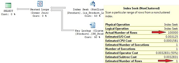
Picture 5: Execution plan created by use of stale statistics

Due to stale statistics, there’s a huge discrepancy between the actual and estimated row-count. The 100000 rows that we’ve added are below the required threshold of 20% modifications; which means that an automatic update isn’t executed. The Index Seek that was used is really not the best choice for retrieving 100000 rows, with additional Key Lookups for every returned key from the Index Seek. The statement took about 300000 logical reads on my PC. A Table or Clustered Index Scan would have been a much better option here.

Solution:

Of course we have the opportunity to provide our knowledge to the optimizer by the use of query hints. In our case, if we knew a Clustered Index Scan was the best choice, we could have specified a query hint, like this:

Although the query hint would do it, specifying query hints is somewhat dangerous. There’s always a possibility that query parameters are modified or underlying data change. When this happens, your formerly useful query hint may now negatively affect performance. An update statistics is a much better choice here:

After that, a Clustered Index Scan is performed and we see only about 86000 logical reads now.

So, please don’t rely solely on automatic updates. Switch it on, but be prepared to support the automatic process by manual updates, probably at off-peak times during your maintenance window. This is especially important for statistics on columns that contain constantly increasing values such as IDENTITY columns. For every added row the IDENTITY column will be set to a value that is above the highest item in the histogram, making it difficult or impossible for the optimizer obtaining proper row-count estimations for such column values. Usually you will want to update statistics on these columns more frequently than only after 20% of changes.

Problem

Filtered statistics pose two very particular problems when it comes to automatic updates.

First, any data modifications that change the selectivity of the filter are not taken into account to qualify for the automatic invalidation of existing statistics.

Second and more important, the “20% rule” is applied to all of a table’s rows, not only to the filtered set. This fact can outdate your filtered statistics very rapidly. Let’s again return to our example with 10% of active data inside a table and a filtered statistics on this portion of the table. If all data of the filtered set have been modified, although this is 100% of the filtered set (the active data), it’s only 10% of the table. Even if we’d change all of the 10% part once again, regarding the table, we only have 20% of data changes. Still our filtered statistics will not be considered as being outdated, albeit we’ve already modified 200% of the data! Please, also keep in mind that this likewise applies to filtered statistics that are linked to filtered indexes.

Solution

For most of the problems I’ve mentioned so far, a reasonable solution involves the manual update or creation of statistics. If you introduce filtered indexes or filtered statistics, then manual updates become even more important. You shouldn’t rely solely on the automatic update of filtered statistics, but should perform additional manual updates rather frequently.

No automatic generation of multi-column statistics

Problem:

If you rely on the automatic creation of statistics, you’ll need to remember that these statistics are always single-column statistics. In many situations the optimizer can take advantage of multi-column statistics and retrieve more exact row-count estimations, if multi-column statistics are in place. You’ve seen an example of this in the introduction.

Solution:

You have to add multi-column statistics manually. If, as a result of some query analysis, your suspect multi-column statistics will help the optimizer, just add them. Finding supportive multi-column statistics can be quite difficult, but the Database Engine Tuning Advisor (DTA) can help you with this task.

Statistics for correlated columns are not supported

There is one particular variation where statistics may not work as expected, because they’re simply not designed to: correlated columns. By correlated columns we mean columns which contain data that is related. Sometimes you will come across two or more columns where values in different columns are not independent of each other; such examples might include a child’s age and shoe size, or gender and height.

Problem:

In order to show why this might cause a problem, we’ll try a simple experiment. Let’s create the following test table, containing a list of rental cars:

This table has two columns, one for the car type and the other one for a daily rate, along with some other data that is of no particular significance for this experiment.

We know that applications are going to query for ‘car type’ and ‘daily rate’, so it may be a good idea to create an index on this columns:

Now, let’s add some test data. We will include four different car types with daily rates adjusted to the car’s type: the better the car, the higher the rate of course. The following script will take care of this:

As you can see, we will have daily rates for luxury cars in the range between $90 and $140, whereas compact cars are given with daily rates between $20 and $39, e.g. In total the script adds 100000 rows to the table.

Now, let’s imagine that a customer asks for a luxury car. Since customers always demand everything to be very low-priced, she doesn’t want to spend more than $90 per day for this car. Here’s the query:

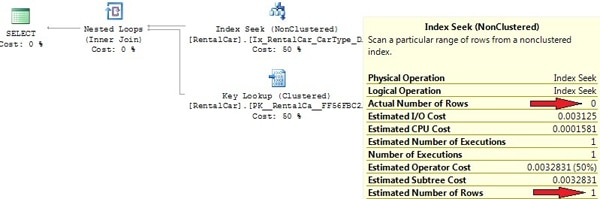
We know that we haven’t a car like this in our database, so the query returns zero rows. But have a look at the actual execution plan (see Picture 6).

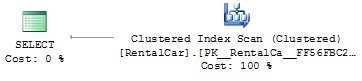
Picture 6: Correlated columns and Clustered Index Scan

Why isn’t our index being utilized here? The statistics are up to date, since we’ve explicitly executed an UPDATE STATISTICS command after inserting the 100000 rows. The query returns 0 rows, so the index is selective and should be used, right? A look at the row-count estimations gives the answer. Picture 7 shows the operator information for the clustered index scan.

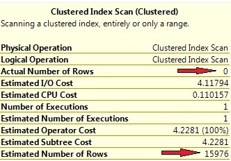
Picture 7: Wrong row-count estimations for correlated columns

Look at the huge discrepancy between the estimated and actual number of rows. The optimizer expects the result set to be of about 16000 rows large, and from this point of view it’s perfectly understandable that a clustered index scan has been chosen.

So, where’s the reason for this strange behavior? We have to inspect the statistics in order to give an answer to this question. If you open the “Statistics” folder inside Object Explorer, the first thing you may notice is an automatically created statistics for the non-indexed column DailyRate. You can then easily calculate the expected number of rows for the condition ‘DailyRate<90’ from the histogram for this statistics (see Picture 8).

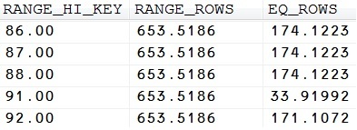
Picture 8: Excerpt from the statistics for the DailyRate column

Just sum up the values for RANGE_ROWS and EQ_ROWS where RANGE_HI_KEY < 90, and you get the row-count for ‘DailyRate < 90’. Actually, ‘DailyRate=89’ would need some special treatment, since this value isn’t contained as a distinct histogram step. Therefore the calculated value won’t be 100% precisely, but it gives you an idea of the way that the optimizer uses the histogram. Of course, we may simply calculate the number of rows by executing the following query:

Look at the estimated row-count in the execution plan, which is 62949.8 in my case. (Your numbers may differ, since we’ve added random values for the daily rate.)

Now we do the same thing with our statistics for the indexed column CarType (see Picture 9 for the histogram).

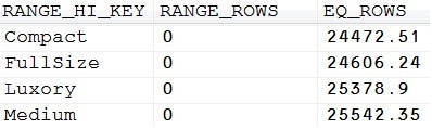
Picture 9: Histogram for the CarType column

Apparently, there are 25378.9 estimated luxury cars in our table. (Note, what a funny thing statistics are! They use two decimal places for exposing estimated values.)

And here’s how the optimizer calculates the cardinality estimation for our SELECT statement:

1. With 62949.8 estimated rows for DailyRate<90, and 100000 total table rows, the density for this filter computes to 62949.8/100000=0.629498.
2. The same calculation is being done for the second filter condition CarType=’Luxory’. This time, the estimated density is 25378.9/100000=0.253789.
3. To determine the total number of rows for the overall filter condition, both density values are simply multiplied. Doing this, we receive 0.629498*0.253789=0.15976. The optimizer takes this value combined with the number of table rows to determine the estimated row-count, which finally calculates to 0.15976*100000=15976. That’s exactly the value that Picture 7 shows.

To understand the problem, you need to recall some school mathematics. By just multiplying the two separate computed densities, the optimizer assumes that values in both participating columns are independent of each other, which apparently isn’t the case. Column values in one column are not equally distributed for all column values in the second column. Mathematically it’s not correct therefore, just to multiply densities (probabilities) for both columns. It’s just wrong to conclude that the total density for ‘DailyRate<90’ for all values of the CarType column will be equally rational for a value of “CarType=’Luxory'”. At the moment, the optimizer does not take column dependencies like this into consideration, but we have some options to deal with this kind of problems, as you’ll see in the following solutions section.

Solution(s):

1) Using an index hint

Of course, we know that the execution plan is unsatisfactory, and this is easy to prove if we force the optimizer to use the existing index on (CarType, DailyRate). We can do this straightforward by adding a query hint like this:

The execution plan will reveal an index seek now. Note that the estimated row-count has not changed however. Since the execution plan is generated before the query executes, cardinality estimations are the same in both experiments.

Nevertheless, the number of necessary reads (monitored with SET STATISTICS IO ON) has been drastically reduced. In my environment I had 5578 logical reads for the clustered index scan and only 4 logical reads, if an index seek is used. The improvement-factor computes to about 1400!

Of course this solution also exposes a great drawback. Despite of the fact that an index hint is apparently helpful in this case, you should generally avoid using index hints (or query hints in general) whenever possible. Index hints reduce the optimizer’s potential options, and may lead to unsatisfactory execution plans when the table data have been changed in a way that the index is no longer useful. Even worse, there’s a chance that the query becomes totally invalid, in case the index has been deleted or renamed.

There are superior solutions, which are presented in the next paragraphs.

2) Using filtered indexes

As of SQL Server 2008, we have the opportunity of working with filtered indexes. That’s quite perfect for our query. Since we only have 4 distinct values for the CarType column, we may create four different indexes, one for every car type. A special index for CarType=’Luxory’ will look as follows:

For the remaining three values of CarType we’d create identical indexes with adjusted filter conditions.

We end up with four indexes and also four statistics that are pretty much adjusted to our queries. The optimizer can take advantage of these tailor-made indexes. You see perfect cardinality estimations along with a flawless execution plan in Picture 10 below.

Picture 10: Improved execution plan with filtered indexes

Filtered indexes provide a very elegant solution to the correlated-columns problem for no more than two participating columns, whenever there are only a handful of values for one contributing column. In case you need to incorporate more than two columns and/or your column values vary widely and unforeseen, you might experience difficulties in detecting proper filter conditions. Also, you should ensure that filter conditions don’t overlap, since this may puzzle the optimizer.

3) Using filtered statistics

I’d like you to reflect on the last section. By creating a filtered index, the optimizer was able to create an optimal plan. Finally it could do so, because we provided it with much improved cardinality estimations. But wait! Cardinality estimations are not gained from indexes. Actually, it’s the index-linked statistics that accounts for the amended appraisal.

So, why not just leave the original index in place and create filtered statistics instead? Indeed that will do it. We can remove the filtered index and create a filtered statistics as an alternative:

If we do the same for the other three values of the CarType column, this again will result in four different histograms, one for each distinct value of this column. Execute our test query again, and you’ll see the same execution plan as the one displayed in Picture 10.

Please be prepared to face identical obstacles, like the ones than were already mentioned in the last section concerning filtered indexes: you may experience difficulties in detecting proper filter conditions.

4) Using covering indexes

I’ve already mentioned that you might face situations where optimal filtered indexes, or statistics are hard to determine. It’ll not always be that easy as in our more educational example. If, you’re unable to uncover subtle filter expressions, there’s another option, you will want to take into consideration: covering indexes.

If the optimizer finds an index where all the required columns and rows can be retrieved from the index without referencing the related table, an index that covers the query, then that index will be used, regardless of cardinality estimations.

Let’s construct an index like that. At first, we remove the filtered statistics to ensure, the optimizer will not rely on this. Afterwards we construct a covering index that the optimizer can benefit from:

If you execute our test query again, you’ll see that the covering index is utilized. Picture 11 displays the execution plan.

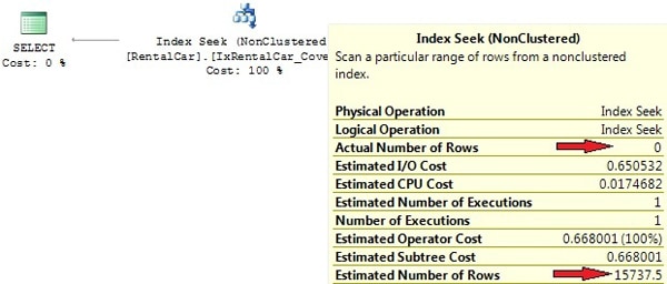
Picture 11: Index Seek with covering index

(Just in case you wonder why we didn’t include the RentalCarID column too, the reason is that we’ve created the clustered index on this column, so it will be included in every nonclustered index anyway.)

Note however that the row-count estimation is still far away from reality! Row-count appraisals are unimportant here. The index is used because our query uses a search argument on the first index column and the index covers the query. One could actually say that the execution plan is just coincidentally efficient.

Please bear in mind that there’s also one special form of a covering index. I’m talking about the clustered index that every table can (actually should) have. If your query is designed in a way that searches on the leading index columns of the clustered index are performed, searching the clustered index will be favorable, irrespective of row-count estimations.

Updates of statistics come at a cost

Problem:

Actually this is not a problem, but just a fact that you have to take into account when planning database maintenance tasks: It’s best to avoid automatic updates of statistics for that 5 million rows table during normal OLTP operations.

Solution(s):

Again, the solution is to supplement automatic updates with manual updates. You should add manual updates of statistics to your database maintenance task-list. Keep in mind, though, that updates of statistics will also invalidate any cached query plans and cause them to be re-compiled, so you don’t want to update too much. If you still face the problem of costly automatic updates during normal operation, you may want to switch to asynchronous updates.

Memory allocation problems

Every query needs a certain amount of memory for execution. The amount of memory required is calculated and requested by the optimizer, where the optimizer takes estimated row-counts and also estimated row sizes into account. If either of the two is incorrect, the optimizer may over- or underestimate the required memory. This is a problem regarding sorts and hash joins. Memory allocation problems may be divided into the following two issues.

An Overestimate of memory requirements

Problem:

With row-count estimations too large, the allocated memory will be too high. That’s simply a waste of memory, since parts of the allocated memory will never get used during query execution. If the system already experiences memory allocation contention, this may also lead to increased wait times.

Solution

Of course the best method is adjusting statistics or re-writing the SQL code. If that’s not possible, you may use query hints (like OPTIMIZE FOR) for providing a better idea of cardinality estimations to the optimizer.

An Underestimate of memory requirements

Problem

That case is even worse! If the requested memory is underestimated, it isn’t possible to acquire additional memory on the fly, that is during query execution. As a result, the query will swap intermediate results to tempdb, causing a performance degrade by factor 8-10!

Solution:

SQL Server Profiler knows the events Errors and Warnings/Sort Warnings and Errors and Warnings/Hash Warnings that will fire, every time a sort operation or hash join makes use of tempdb. Whenever you see this happen, it’s probably worth further investigations. If you suspect underestimated row-counts as the cause for tempdb swapping, see if updating statistics or SQL review and edit will help. If not, consider query hints for solving the issue.

Additionally, you may also increase the minimum amount of memory that a query allocates by adjusting the configuration option min memory per query (KB). The default is 1 MB. Please make sure that there’s no other solution before you opt for this. Every time you change configuration options, it’s good knowing exactly what you’re doing. Modifying configuration options should generally be your last choice in solving problems.

Best practices

I’ve extracted all of the advices given so far and put them into the following best practices list. You may consider this as a special kind of summary.

• Be lazy. If there are automatic processes for creating and updating statistics, make use of them. Let SQL Server do the majority of the work. The option of automatically creating and updating statistics should work out fine in almost all cases.
• If you experience problems with query performance, this is very often caused by stale or poor quality statistics. In many situations you won’t find the time for deeper analysis, so simply perform an update statistics first. Be sure not to do this update for all existing tables, but only for the participating tables or indexes of poor performing queries. If this doesn’t help, you may be the point at which you consider updating distinct statistics with full scan. Watch out for differences between actual and estimated row-counts in the actual execution plan. The optimizer should estimate, not guess! If you see considerable differences, this is very often an indicator for non-conforming statistics – or poor TSQL code, of course.
• Use the built-in automatic mechanisms, but don’t rely solely on these. This is particularly true for updates. Support automatic updates through additional manual ones, if necessary.
• Rebuild fragmented indexes when necessary. This will also update existing index-linked statistics with full scan. Be sure not to update those index-linked statistics again right after an index rebuild has been performed. Not only is this unnecessary, it will even downgrade those statistics’ quality if the default sample rate is applied.
• Carefully inspect, if your queries can make use of multi-column statistics. If so, create them manually. You may utilize the Database Engine Tuning Advisor (DTA) for regarding analysis.
• Use filtered statistics when you need more that just 200 histogram entries. When introducing filtered statistics, you will want to perform manual updates; otherwise your filtered statistics might get stale very soon.
• Don’t create more than one statistics on the same column unless, of course, they are filtered statistics. SQL Server will not prevent you from generating multiple statistics for one column: Likewise, you can have several identical indexes on the same column. Not only will this increase the maintenance effort, it will also increase the optimizer’s workload. Moreover, since the optimizer will always use one particular statistics for estimations of cardinality, it has to choose one statistics out of a set. It will do this by rating statistics and selecting the “best” one. This could be the one with the newest last update date, or perhaps the one with a larger sample size.
• And last but not least: improve your TSQL Code. Avoid using local variables in TSQL Scripts or overwriting parameter values inside stored procedures. Don’t use expressions in search arguments, joins, or comparisons.