Why should we be interested in SQL Server Statistics, when we just want to get data from a database? The answer is ‘performance’. The better the information that SQL Server has about the data in a database, the better its choices will be on how it executes the SQL. Statistics are its’ chief source of information. If this information is out of date, performance of queries will suffer.

Contents

Introduction

The SQL queries that you execute are first passed to the SQL Server Query Optimizer. If it doesn’t have a plan already stored or ‘cached’, it will create an execution plan. When it is creating an execution plan, the SQL Server optimizer chooses an appropriate physical operator for any logical operation (such as a join, or a search) to perform. When doing so, the optimizer has some choice in the way that it maps a distinct physical operator to a logical operation. The optimizer can, for example, select either a ‘physical’ Index Seek or Table Scan when doing a ‘logical’ search, or could choose between a Hash, – Merge-, and Nested Loop joins in order to do an inner join.

There are a number of factors that influence the decision as to which physical operators the optimizer finally chooses. One of the most important ones are cardinality estimations, the process of calculating the number of qualifying rows that are likely after filtering operations are applied. A query execution plan selected with inaccurate cardinality estimates can perform several orders of magnitude slower than one selected with accurate estimates. These cardinality estimations also influence plan design options, such as join-order and parallelism. Even memory allocation, the amount of memory that a query requests, is guided by cardinality estimations.

In this article we will investigate how the optimizer obtains cardinality estimations by the use of statistics, and demonstrate why, to get accurate cardinality estimates, there must be accurate data distribution statistics for a table or index. You will experience how statistics are created and maintained, including what problems can occur, such as which limits you have to be aware of. I’ll show you what statistics can do, why they are good, and also where the statistics may not work as expected.

Prerequisites

Engineer that I am, I love experimenting. Therefore, I have carefully prepared some experiments for clarifying and illustrating the underlying concepts. If you want to follow up these experiments, you will want to create a separate database with a Numbers table first. The following script will create the sample database and table:

The Numbers table is very useful as a row provider in a variety of cases. I’ve first started working with a table of this kind after reading [1]. If you’re like me, you’ll fall in love with this table very soon! Thank you, Itzik!

Statistics and execution plan generation

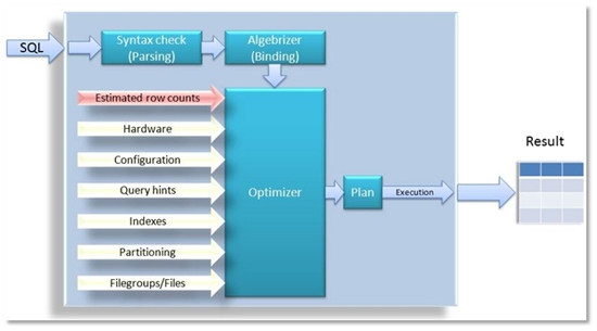
Picture 1: Query optimization process

A SQL query goes through the process of parsing and binding and finally a query processor tree is handed over to the optimizer. If it only had this information about the Transact-SQL to perform, however, the optimizer would not have many choices for determining an optimal execution plan. Therefore, additional parameters are considered, as you can see in Picture 1:  Even some information about hardware, such as the number of CPU-cores, system configuration or the physical database layout also affects the optimization and the generated execution plan. Every single parameter that are listed as arrows in Picture 1 are relevant to the optimizing process, and therefore affect the overall performance of queries. Cardinality estimations probably have the most influence on the chosen plan.

Picture 1 is slightly inaccurate in that it shows that cardinality estimations are provided to the optimizer. This is not quite exact, because the optimizer itself may consider the maintenance of relevant row count estimations.

Introductory Examples

To illustrate some of these points, we will use a table with 100001 rows, which is created by executing the following script:

As you can see, we insert 100000 rows with a value of 1000 for column c1 into table T0, and then only one additional row with a value of 2000.

With that table at hand, let’s have a look at the estimated execution plans for the following two queries:

You will see two different execution plans. Have a look at picture 2 to see, what I’m talking about.

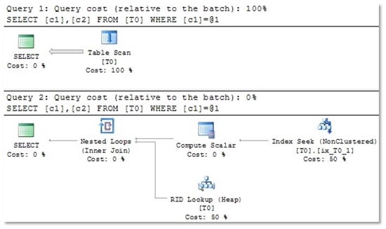
Picture 2: For the first query, which will return 100000 rows, the optimizer chooses a Table Scan. The second query yields only one single row, so in this case, an Index Seek is very efficient.

It looks as if the execution plan depends on the value used for the comparison. For each of the two used values (1000 and 2000) we get a tailor-made execution plan.

But how can this happen? Have a look at the estimated row counts for the Scan and Seek operators. You can do so by hovering with the mouse above these operators. Inside the popup window, you will find different row count estimations for each of the two queries (see Picture 3).

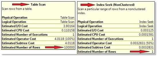
Picture 3: Estimated row counts

Clearly, the plan is adjusted to these row count estimations. But how does the optimizer know these values? If your educated guess here is “due to statistics”: yes, you’re absolutely right! And, surprisingly, the estimated number of rows and the actual number of processed rows are exactly the same! In our case, we can check this easily just by executing the two queries. In fact, we know about the number of processed rows already in advance of the query execution, because we’ve just inserted the rows. But you certainly can imagine that it’s not always that easy. Therefore, in many cases, you will want to include the actual execution plan as well. The actual execution plan also contains information about the actual number of rows – those rows that were really processed by every operator.

Now, let’s investigate the actual execution plan for the following query:

Not surprisingly, we see an Index Seek operator on the top right, just as the second plan in Picture 2 shows. The information for the Index Seek operator in the actual plan, however, is slightly extended compared with the estimated execution plan. In Picture 4 you can see that, this time, additional information about the actual number of rows can be obtained from the operator information. In our example the estimated, and actual, row count differs slightly. This has no adverse impact on performance, however, since an Index Seek is used for returning 0 rows, which is quite perfect…

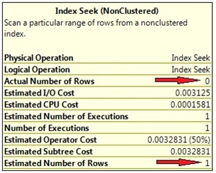
Picture 4: Estimated and actual row counts.

Now, finally let’s have a look at the actual execution plan for this query:

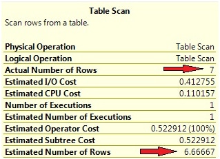
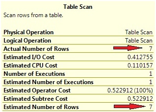
As we have only one single row with a value of 2000 for c1, you will expect to see an Index Seek here. But surprisingly, a full Table Scan is performed, which is not really a good choice. I’ll explain to you later, why this happens. As for now, have a look at the operator information, shown in Picture 5.

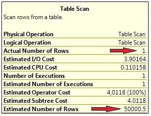
Picture 5: Large discrepancy between estimated and actual row count

You can see that the estimated row count is considerably different from the actual number of processed rows. As the plan is, of course, created before the query can be executed, the optimizer has no idea about the actual number of rows during plan generation. In order to compile the optimizer assumes that about 50000 rows are returned. From this perspective it is very clear why a Table Scan is chosen: for this large number of rows, the Table Scan is just more efficient than an Index Seek. So we end up with a sub-optimal execution plan in this case.

Under the hood

So, why do we need statistics in order to estimate cardinality? There’s a simple answer to that question: statistics reduce the amount of data that has to be processed during optimization. If the optimizer had to scan the actual table or index data for cardinality estimations, plan generation would be costly and lengthy.

Therefore, the optimizer refers to samples of the actual data called the statistics, or distribution statistics. These samples are, by nature, much smaller than the original amount of data. As such, they allow for a faster plan generation.

Hence, the main reason for statistics is to speed up plan generation. But of course, statistics come at a cost. First, statistics have to be created and maintained, and this requires some resources. Second, the information held in the distribution statistics is likely to become out-of-date if the data changes, so we have to expect common redundancy problems such as change anomalies. As statistics are stored separately from the table or index they relate to, some effort has to be taken to keep them in sync with the original data. Finally, statistics reduce, or summarize, the original amount of information. We know that, due to this ‘information reduction’, all statistical information involves a certain amount of uncertainty or, as Aaron Levenstein once said:

“Statistics are like bikinis. What they reveal is suggestive, but what they conceal is vital.”

Whenever a distribution statistic no longer reflects the source data, the optimizer may make wrong assumption about cardinalities, which in turn may lead to poor execution plans.

Statistics serve as a compromise between accuracy and speed. Statistics enable faster plan generation at the cost of their maintenance. If the maintenance is neglected, then this increases the risk of an inaccurate query plan.

General organization of statistics

The following script creates another test table which we’ll use to see in which manner statistics affect query optimization:

By running the script above we will obtain a table with four columns, 100000 rows, and a non-clustered index on column x.

Obtaining information about statistics

Achieving information about statistics using Management Studio

You may open our test table T1 in Object Explorer and find an entry “Statistics” when expanding the folder for the table “dbo.T1” (see Picture 6).

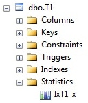
Picture 6: Display of statistics in SSMS Object Explorer

At the moment, there’s one single statistics object with the same name as our non-clustered index. This statistics object has been automatically created at the time that the index was generated. You will find a statistics object like this for every existing index. During index creation or rebuild operations, this statistics object is always refreshed, but it is not done in the course of reorganizing an index. There is one peculiarity with those index-related statistics: if an index is created or rebuilt via CREATE INDEX or ALTER INDEX … REBUILD the sample data that flows into the linked statistics is always obtained by processing all table rows. Apparently, for the index generation, all table rows have to be processed anyway. Consequently, the statistics object is created by using all these rows. Usually, this is not the case. In general, for larger tables, only some randomly chosen data are used for the underlying sample. Only for smaller tables, a full scan will always be performed.

SSMS Object Explorer allows the examination of detailed information about a statistics object by opening the properties window. The “General” page provides some data about covered columns and the point in time of the last update. You may also trigger an instant statistics update by selecting the relevant check box.

More interesting data is shown on the “Details” page. Here you will find detailed information about data distributions. Picture 7 shows a sample of what you might see on this page.

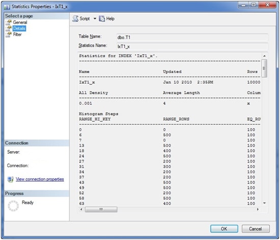
Picture 7: Statistics Details Window

Right below the name of the statistics, there are three main areas of information (which unfortunately, do not completely fit inside the provided screen shot):

1. General information. In this area you can see information regarding the statistics’ creation, and the total number or rows the index encompasses. Also, the number of samples that have been taken from the table for the generation of the histogram is included (see below for an explanation of the histogram).
2. All Density. This value represents the general density of the entire statistics object. You may simply calculate this value by the formula:1/(distinct values) for the columns comprising the statistics. For single column statistics (as in our example) there’s only one row. For multi column statistics, you’ll see one row for each left based subset of the included columns. Let’s assume we have included three columns c1, c2, and c3 in the statistics. In this case, we’d see three different rows (All Density values): one for (c1), a second one for (c1, c2), and finally a third one for (c1, c2, c3). In our example there’s a single column statistics for column x, so there’s only one row. There are 1000 distinct values for column x, so the All Density calculates to 0.001. The optimizer will use the ‘All Density’ value whenever it is not possible to get a precise estimation from the histogram data. We’ll come back to this a little later.
3. Histogram. This table contains the sample data that has been collected from the underlying table or index. Inside the histogram, the optimizer can discover a more or less exact distribution of a column’s data. The histogram is created and maintained (only) for the first column of every statistics – even if the statistics is constructed for more than one column.
   The histogram table will never encompass more than 200 rows. You can find the number of steps inside the first section, containing the general information.
   The histogram columns have a meaning as follows:

Column	Description
RANGE_HI_KEY	This is the column value at the upper interval boundary of the histogram step.
RANGE_ROWS	This is the number of rows inside the interval, excluding the upper boundary.
EQ_ROWS	The value represents the number of rows at the upper boundary (RANGE_HI_KEY). If you like to know the number of rows, including the lower and upper boundary, you can add this value and the number presented through the RANGE_ROWS value.
DISTINCT_RANGE_ROWS	This is the number of distinct interval values, excluding the upper boundary.
AVG_RANGE_ROWS	The value presents the average number of rows for every distinct value inside the interval, again excluding the upper boundary. Hence, this is the result of the expression RANGE_ROWS / DISTINCT_RANGE_ROWS (where DISTINCT_RANGE_ROWS < 0).

Table 1: Histogram columns

Obtaining information about statistics using Transact-SQL

SQL Server provides a large number of system views for retrieving much information on its inner workings. Information regarding statistics is no different. You can use two main system views for viewing information about existing statistics. The sys.stats view delivers general facts. You’ll see one row for every statistics object. By using the second view, sys.stats_columns, you can have a look at the statistics columns, as the name of this view suggests. The following query will return all existing statistics for every user table inside the selected database:

The three columns show table and name of the statistics object, as well as the moment of the last update.

Unfortunately, there’s no system view for querying histogram data. If you like to see a statistics’ histogram, you’ll have to use DBCC with the SHOW_STATISTICS option like this:

yields detailed information on the three areas that you already have seen in Picture 7.

By using the optional WITH clause, there’s also a possibility of showing just portions of the information that is available. For example, by using WITH HISTOGRAM, you’ll see only histogram data and the other parts are left out.

Finally, we also have the stored procedure sp_helpstats. This SP will yield general information for statistics on a table. It expects the table’s name as parameter. The returned information is very unsubstantial, however, and maybe that’s the reason why Microsoft had deprecated this stored procedure.

A more detailed look at the utilization of statistics

So far, we have created a test table T1 with one index and one statistics (see Picture 7). Now, let’s dig a little deeper and see how our existing statistic is used. For the beginning, we start with a very simple statement:

The actual execution plan can be seen in Picture 8.

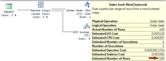
Picture 8: Actual execution plan

It shows an Index Seek (NonClustered) with an estimated row count of 100, which is quite accurate, isn’t it? We are now able to determine how the optimizer computes this estimation. Have a look at the statistics for the utilized index IxT1_x. Picture 9 reveals an excerpt from the histogram (obtained by using DBCC SHOW_STATISTICS).

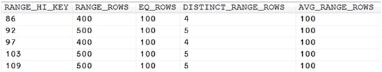
Picture 9: Excerpt from the histogram for statistics IxT1_x

We are querying all rows for a value of x=100. This particular value falls in between the interval bounds 97…103 of the histogram. The average number of rows for each distinct value inside this interval is 100, as we can see in the histogram’s AVG_RANGE_ROWS. Since we are querying all rows for one distinctive value of x only, and, from the statistics it appears that there is on average 100 rows for each specific value of x inside this interval, the optimizer estimates that there are 100 rows for the value of x=100. That’s an excellent estimate, as it concurs precisely with the actual value. The existing histogram works well.

Now have a look at the following query:

Not surprisingly, you will see a Table Scan in the execution plan, as there is no index on column a (see Picture 10).

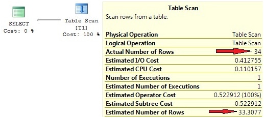
Picture 10: Row count estimation for non-indexed column

The interesting thing here is the “Estimated Number of Rows”, which again is quite exact. How does the optimizer know this value? We don’t have an index for column a, hence there aren’t any statistics. So, where does this estimation come from?

The answer is quite simple. Since there is no statistics, the optimizer will automatically create the missing statistics. In our case, this statistic is created before the plan generation commences, so plan compilation will take slightly longer. There are other options for generation of statistics, which I’ll explain a little further down.

If you open the Statistics folder for table T1 in object explorer, you’ll see the auto-created stats (look at Picture 11).

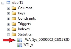
Picture 11: Automatically created statistics

Auto-created statistics are easily revealed by their automatically created name, which always starts with “_WA”. The sys.sys_stats view has a column called auto_created that differentiates between automatically and manually created statistics. For index-related statistics, this column will show a value of “false”, even though these statistics are auto-generated as well.

SSMS exposes a problem when it comes to the presentation of detailed data for statistics that are not linked to an index. You will see no detailed data (and thus, no histogram) for these statistics. So, don’t expect to see something like shown in Picture 7 for “pure” column statistics. The good news is that we have an option here: DBCC SHOW_STATISTICS. If you like to see histogram data, make use of this command.

You might wonder what statistics for non-indexed columns are useful for. After all, the only possible search operation is a scan in this case, so why bother about cardinality estimations? Please remember that cardinality estimations not only affect operator selection. There are other issues that are determined by row-count estimations. Samples include: join order (which table is the leading one in a join operation), the utilization of spool operators, and memory grants for things like hash joins and aggregates.

We currently have statistics for columns a (auto created, no related index) and x (linked to index IxT1_x). Both statistics are useful for queries that filter on each of the two columns. But what if we use a filter expression with more that only one column involved? What happens, if we execute the following query?

Row count estimations in the actual execution plan look like shown in Picture 12.

Picture 12: Row count estimation for multi-column filter expression

This time, the estimated and actual values differ. In our example, the absolute difference is not dramatic, and doesn’t spoil the generated plan. A Table Scan is the best (actually the only) option for performing the query, since we have no index on either of the two columns, a and b, that are used in the predicate. But there may be circumstances where those differences are vital. I’ll show you an example in the second part of this article, when we talk about problems with statistics.

The reason for the discrepancy lies in the method for automatically creating statistics. These statistics are never created for more than one column. Although we are filtering on two columns, the optimizer will not establish multi-column statistics for columns (a, b) or (b, a) here. It will only add one single column statistics for column b, since this one does not yet exist. So, the optimizer ends up with two separate statistics for columns a and b. For cardinality estimations, the histogram values for both statistics are combined in some way. I’ll explain in detail, how this works a little later. As for now, we can only suppose that this process is somehow fuzzy. But of course, we’re talking about estimated values here, which usually will not match exactly with real values (as it was the case in our first experiments).

Nevertheless, you may object that a multi-column statistics would have led to improved estimations here. If the optimizer does not create multi-column statistics, why not do this manually? For this task we can use the CREATE STATISTICS command, as follows:

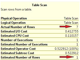
Now, when we execute our last statement again, the estimated row count has improved significantly (see Picture 13).

Picture 13: Row count estimations with multi column statistics

The two plans itself show no differences, so in our simple case the improved estimation has no impact. But it’s not always that easy, so you might consider using multicolumn statistics under certain circumstances.

Please keep in mind that the histogram is always only created for the leading column. So, even with multicolumn statistics, there’s only one histogram. The reason for this practice becomes obvious when you consider the sample size again. Remember that the maximum number of rows in a histogram is 200. Now, imagine a two column statistics with separate histograms for each column. Apparently, for each of the 200 samples for the first column, a separate sample for the second column had to be established, so the total sample size for the statistics, as a whole, would equal 200 * 200 = 40,000 samples. For three columns, we’d have already 8,000,000! Doing so would really outweigh the benefits of statistics, namely information-reduction and increasing the speed of plan compilation. In many cases, statistics would really impede the optimization process.

Statistics generation and maintenance

Statistics represent a snapshot of data samples that have come from a table or index at a particular time. They must be kept in sync with the original source data in order to allow suitable cardinality estimations to be made. We will now examine some more of the techniques behind statistics generation and synchronization.

Creation of statistics

You can have your statistics creation done automatically, as is generally the preferable choice. This option is set at the database level, and if you didn’t modify your model database in this respect, all of your created databases will have set the AUTO CREATE STATISTICS option to ON initially.

You may query, and set, this option through SSMS. Just open the properties window for your database and switch to the “Options” page. Inside the “Automatic” group you will find the relevant settings (see Picture 14).

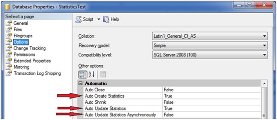
Picture 14: Statistics options at the database level

There are three options regarding statistics. As for now, we’re only interested in the first one,”Auto Create Statistics”, which will turn the automatic statistics creation on or off. I’ll explain the other two options in the next section.

Of course, you may also turn the auto-create mechanism on and off using the ALTER DATABASE command, like this:

If you turn off the automatic generation option, your statistics will no longer be created for you by the optimizer. Statistics that belong to an index are not affected by this option, however. As already mentioned, those statistics will always be automatically created during index generation or rebuild.

I suggest setting this option to on, and let SQL Server take care of creating relevant statistics. If you, for whatever reason, don’t like the automatic mode, you have to create statistics on your own. I’ll show you some examples of cases where you might prefer creating statistics manually in some cases, in part two of this article. By no means should you should decide to not use statistics at all. If you opt for working with manually created statistics, there are two options for creating them. The first possibility, which you already know, is the CREATE STATISTICS command. You can create statistics, one-by-one by executing CREATE STATISTICS, which can be painful. Therefore, you may consider another option: sp_createstats. This stored procedure will create single-column statistics for all columns in all of your tables and indexed views, depending on options selected. Of course, you are free to use this procedure along with the AUTO CREATE STATISTICS option set to ON. But be aware that there’s a chance you end up with a bunch of statistics that never get used, but will have to be maintained (kept in sync with source data). Since we don’t have any usage information for statistics, it’s almost impossible to detect which of your statistics the optimizer takes advantage of. On the other hand, the chance that the optimizer comes across a missing statistics at run time of a query will be minimized, so missing statistics won’t have to be added as part of the optimization process. This may lead to faster plan compilations and overall increased query performance.

Sometimes it’s useful to monitor ‘auto-stats’ creation, and this is where SQL Server Profiler comes into play. You can add the event Performance/Auto Stats to watch out for the creation and updating of your statistics. There’s a chance that you see longer query execution times whenever this event occurs, since the statistics object has to be created before an execution plan can actually be generated. Because the automatic creation and updating of statistics will usually occur without warning, it can be hard to determine why a particular query was performing very poorly, but only at a particular execution or particular point in time. So this is an argument for creating your statistics manually. If you know which statistics will be useful for your system; you may create them manually, so they won’t have to be added at run time. But leave the AUTO CREATION option set to ON nevertheless, so the optimizer may add missing statistics that you haven’t been aware of.

CREATE STATISTICS gives you an extra option to specify the amount of data that is processed for a statistics’ histogram that you don’t have to when relying on auto generation. You may specify an absolute or relative value for the number of rows to process. The more rows that are processed, the more precise your statistics will be. On the other hand, doing full scans in order to deal with all existing rows and create high-quality statistics will take a longer time, so you have to trade-off between statistics quality and utilized resources for statistics creation.

Here’s an illustration of how the sample size may be quantified:

If you don’t specify the sample size, the default setting is used. This should be appropriate in most cases. I’ve seen that, for smaller tables, a full scan is always used, regardless of the specified sample size. Also, be aware that the provided sample size is not always used, as only whole data pages are being processed, and always all rows of one read data page are incorporated into the histogram.

Keep in mind that automatically-created statistics are always single-column statistics. If you like to take advantage of multi-column statistics, you have to create them manually. There’s another reason for creating statistics manually, which takes us to the next section: filtered statistics.

New in SQL Server 2008: filtered statistics

SQL Server 2008 introduces the concept of filtered indexes. These are indexes that are created selectively, that is, only for a subset of a table’s rows. Whenever you create a filtered index, a filtered statistic is also created. Moreover, you may also decide to create filtered statistics manually. As a matter of fact, if you like to try using filtered statistics, you’ll have to create them manually, since automatic creation always generates unfiltered statistics.

So, why would you like your optimizer to work with filtered statistics? In general, filtered statistics allow more than one statistics for the same column, but for different rows. Thereby, the following capabilities are available:

1. Advanced granularity: Please remember the sample size of the histogram, which is limited to 200 steps. Sometimes this might not be sufficient. Imagine a table with one billon rows, providing only 200 samples to the optimizer for cardinality estimations. This can be far too few. Filtered statistics offer a simple opportunity for increasing the sample size. Just create multiple statistics, ideally with mutually exclusive filter restrictions, so the different histograms won’t overlap. In doing so, you originate 200 samples for every statistics, which obviously increases the statistics’ granularity for the table as a whole and allows for more exact row count estimations.
2. Statistics tailored to specific queries. If you have a monster killing query slowing down your application every time it runs, you will have to handle this in some way. The creation of specific statistics for a particular support of this query could also be part of a solution. Filtered statistics increase the capabilities for such adjustments. You’ll see a basic example for this a little further down.
3. Statistics for partitioned tables. If you allocated a table into different partitions, you probably did so for good reasons. Maybe, you have a large table containing 90% infrequently queried historical data and only 10% of current data that is regularly queried during normal operations. You may want to split this table into two partitions, arranged according to the access patterns. Be aware, however, that statistics are not automatically filtered to match created partitions. By default, statistics are always unfiltered, so automatically created column statistics cover the whole table across all partitions. It may be a good idea to adjust your statistics in a way that they correspond to your partitions. If you did so in our example, you had one histogram for a relatively small portion of the table (10% of table data). Apparently this histogram was of higher quality than one for the table as a whole, and therefore your frequently executed queries could profit from improved cardinality estimations.
4. Decreased maintenance effort for updating statistics. Think again about our last example with a separate statistics for the frequently used and rather small current table data. Usually, the historical part of the table experiences no updates, so the statistics for this portion never needs updating after creation. Only statistics for 10% of the table’s data will have to be updated, which may cut the overall resource usage for updating statistics. (I say “may”, since every update for this part of statistics will need fewer resources, but usually will occur more often.) I’ll explain this a little deeper in the problems section at the end of the second part of this article series.

Let’s try a simple example. For this example we borrow the following query from a previous experiment:

You can have a look at the actual execution plan in Picture 13. Now, in order to improve the estimated row counts even further, we decide to create a filtered statistics object. We’re going to filter on one of the two columns used in the WHERE condition and create the statistics on the other column. This can be very simply accomplished by adding the WHERE clause to the CREATE STATISTICS statement:

So this time the statistics is custom-made in respect to our query, and indeed we observe exact row count estimations, as the actual execution plan exposes (see Picture 15).

Picture 15: Filtered statistics and execution plan

You see that filtered statistics can help the optimizer, if they are carefully chosen. Unfortunately, it isn’t easy to detect which filtered statistics the optimizer really can take advantage of. You will have to do this by hand which can be fairly painful and also requires some experience. The Database Engine Tuning Advisor will not help you in the process of discovering appropriate filtered statistics, since the creation of filtered statistics is not included into DTA’s analysis. As I said: you will have to do this manually!

Also, please be aware that filtered statistics may come at the cost of increased maintenance. If you use filtered statistics for an increased sample size of the histogram, you end up with more statistics and more samples than in the “unfiltered circumstance”. All of these additional statistics have to be kept in sync with the table data. This is another reason for an intensified maintenance effort. Remember, if AUTO CREATE STATISTICS is set to ON, always unfiltered column statistics will be added, if they are missing. Whenever the optimizer comes across a missing unfiltered statistics for a column, it will add an unfiltered statistics for that column, regardless of an already existing filtered statistics that covers the query. So, with manually created filtered statistics and AUTO CREATE STATISTICS set to ON, you will have to maintain filtered and non-filtered statistics. This is unlikely to be what you want.

Talking about maintenance, we’re now ready to discover how existing statistics can be properly maintained.

Updating statistics

I’ve already mentioned that statistics only contain redundant data that have to be kept in sync with original table or index data. Of course, it’d generally be possible to revise statistics on the fly, in conjunction with every data update, but I think you agree that doing so would negatively affect all update operations.

Therefore, the synchronization is decoupled from data change operations, which of course also means that you have to beware of the fact that statistics may lag behind original data and are always somewhat out of sync.

SQL Server allows two possibilities of keeping your statistics (almost) in sync. You can leave the optimizer in charge for this task and rely on automatic updates, or you may decide to update your statistics manually. Both methods include advantages and disadvantages and may also be used in combination.

Automatic updates

If you’d like to leave the optimizer in charge of statistics updates, you can generally choose this option at the database level. Picture 14 shows how you may set the AUTO UPDATE STATISTICS with the help of SSMS. Of course, there are also corresponding ALTER DATABASE options available, so you may switch the automatic update on and off via Transact-SQL as well:

As Picture 14 and the regarding TSQL commands above reveal, SQL Server offers two different approaches of automatic updating:

1. Synchronous updates. If the optimizer recognizes any stale statistics, when creating or validating a query plan, those statistics will be updated immediately, before the query plan is created or recompiled. This method ensures that query plans are always based on current statistics. The drawback here is that plan generation and query execution will be delayed, because they have to wait for the completion of all necessary statistics’ updates.
2. Asynchronous updates. In this case, the query plan is generated instantaneously, regardless of any stale statistics. The optimizer won’t care about having the latest statistics at hand. It’ll just use statistics as they are right at the moment. However, stale statistics are recognized, and updates of those statistics are triggered in the background. The update occurs asynchronously. Obviously, this method ensures for faster plan generation, but may originate only sub-optimal execution plans, since plan compilation may be based on stale statistics. Asynchronous updates are available only as an additional option of the automatic statistics update, thus you can only enable this setting with AUTO UPDATE STATISTICS set to ON.

The above methods offer both advantages and disadvantages. I usually prefer synchronous updates, since I like my execution plans to be as exact as possible, but you may experience improved query performance when you chose ‘asynchronous’. After SQL Server installation, the default (and also recommended) setting is automatic and synchronous updates, so if you didn’t change your model database, all of your created databases will have this option initially configured.

Of course, there’s one open question. If the optimizer is able to discover outdated statistics, what are the criteria for the decision, whether a particular statistics needs a refresh? Which measures are taken into consideration by the optimizer for the evaluation of a statistics’ correctness?

SQL Server has to know about the last update of statistics and subsequent data changes in order to detect stale statistics. In earlier versions of SQL Server, this monitoring was maintained at row granularity. Beginning with version 2005, SQL Server now monitors data changes on columns that are included in statistics by maintaining a newly introduced, so called colmodctr for those columns. The value of colmodctr is incremented every time a change occurs to the regarding column. Every update of statistics resets the value of colmodctr back to zero.

By the use of the colmodctr column and the total number of rows in a table, SQL Server is able to apply the following policies to determine stale statistics:

• If the table contained more than 500 rows at the moment of the last statistics update, a statistics is considered as to be stale if at least 20% of the column’s data and additional 500 changes have been observed.
• For tables with less or equal than 500 rows from the last statistics update, a statistic is stale if at least 500 modifications have been made.
• Every time the table changes its row count from 0 to a number greater than zero, all of a table’s statistics are outdated.
• For temporary tables, an additional check is been made. After every 6 modifications on a temporary table, statistics on temporary tables are also invalidated.
• For filtered statistics the same algorithm applies, regardless of the filter’s selectivity, however. Column changes are always considered for the entire table, the filtered set is not taken into account. You can easily get trapped by this behavior, as your filtered statistics may “grow old” very fast. I’ll explain this more detailed in the problems part at the end of part two of this article.

Unfortunately, colmodctr is kept secret and not observable, through DMVs. Therefore, you can’t watch your statistics in order to uncover those statistics that are likely to be refreshed very soon. (Well, actually you can by connecting via the dedicated administrator connection (DAC) and utilizing undocumented DMVs, but let’s just forget about undocumented features and say we don’t have access to colmodtr values.)

It’s a common misconception that statistics will be updated automatically whenever the necessary numbers of modifications have been performed, but this is not accurate. Statistics are automatically updated only when it is necessary in order to get cardinality estimations. If table T1 contained 100 rows and you insert a million further rows, you’ll experience no auto-update statistics during those INSERT operations, but existing statistics will be marked as stale. There’s no need for update statistics until cardinality estimations for table T1 have to be made. This will be necessary for instance, if the table is used inside a join, or if one of the columns is used in a WHERE condition.

If you experience problems with too many updates of statistics, you may wish to prevent certain tables or even statistics from automatic updates. I remember a case where we had a table that was used as a command queue. This table had no more than a few rows (by all means less than 500) at any point in time, and usually the command queue was empty quite often and changed very rapidly, since we’ve processed quite a few commands per second. Every successful processed command was deleted from the queue immediately: Therefore, the row count for this table changed from zero to one quite often. According to the rules I’ve mentioned above, every time this happened, statistics for this particular table were classified as stale and got updated whenever a command was retrieved from the queue. We were always querying commands from this table via the clustered index, which in this case also represented the primary key, so there was no need to update statistics at all. The optimizer would use the clustered index anyway, which is what we wanted.

There’s a stored procedure called sp_autostats, which lets you exclude certain tables, indexes or statistics from the automatic updates. So, you can have the AUTO UPDATE STATISTICS set to ON at the database level to be sure, the optimizer can operate with current statistics. If you identify problems with too many updates for certain tables, like in the example above, you can switch the automatic mode off selectively. The CREATE STATISTICS command also offers a solution, if you create statistics manually. This command understands a NORECOMPUTE option that you can apply, if you create a statistics manually and don’t want to see automatic updates for this statistics. Likewise, the CREATE INDEX command has an option STATISTICS_NORECOMPUTE than can be switched on, if you don’t like to experience automatic updates for the index-linked statistics.

Manual updates

If we have an automatic mode, why would we bother about manual updates at all? Wouldn’t it be easier to rely on the automatic process and let SQL Server deal with updates of statistics?

Yes, this is almost the case. The automatic update is fine in many cases. It ensures your statistics are current, which apparently is what you should be after. But you may also face times when it makes sense to updated statistics manually. Some of the reasons are covered in the problems section below, but here’s an outline:

• I’ve already mentioned that you may decide to exclude statistics from automatic updates. If you do so, instead of never updating those statistics, you could also perform occasional manual updates. This might be best, for example, after bulk loads into a table that experiences no changes beside those bulk loads.
• Remember that for tables with a relevant number of rows, statistics are updated automatically only after about 20% of the table’s data were modified. This threshold could be slightly too high. Therefore, you might decide to perform additional manual updates. I’ll explain a circumstance where this would be the case in part 2.
• If you rely on the automatic update of statistics, a lot of those updates may happen during operational hours and adversely affect your system’s performance. Asynchronous updates provide one solution to this, but it may also be a good idea performing updates of stale statistics at off-peak times during your nightly maintenance window.
• The automatic update will create a histogram only by applying the default, and limited, sample size. Increasing the sample size for selected statistics, and thus the quality of the statistics, may be necessary if you experience performance problems. If you’d like distinct statistics to be updated with sample size set to full e.g., so all of a table’s rows are processed for the histogram, you will have to perform the update manually.
• If you use filtered statistics, you have to be aware that the definition of ‘stale’ says nothing about the selectivity of the filter. If changes occur that modify the selectivity of any of your filters, you very likely have to perform manual updates of those statistics.
• There’s another issue with filtered stats, as the automatic update is very likely to be less than perfect. Trust me; you will want to support automatic updates through manual refreshes when using filtered statistics. You’ll get a deeper explanation of this in part two of this article.

If you plan for manual updates, there are two options. You can use the UPDATE STATISTICS command or the stored procedure sp_updatestats.

UPDATE STATISTICS allows specific updates of distinct statistics, as well as updates of all existing statistics for a table or index. You may also specify the sample size, which is the amount of table data that is processed for updating the histogram. The somewhat simplified syntax looks like this:

Besides using the FULLSCAN option, which will produce high quality statistics, but may consume a lot of resources, UPDATE STATISTICS also allows the specification of the sample size in terms of the percentage of a table’s data, or by itemizing the absolute number of rows to process. You may also direct the update to rely on the provided sample size that has been specified in a prior CREATE or UPDATE STATISTICS operation. Here are some examples:

Update all statistics tor table T1 with full scan:

Update all column statistics (that is, statistics without a related index) for table T1 by using the default sample size and exclude those statistics from further automatic updates:

Update statistics s1 on table t1 by processing 50 percent of the table’s rows:

When you decide for manual updates of statistics, please keep in mind that index-rebuild operations also update statistics that are related to a rebuilt index. As an index rebuild will always have to handle all table rows, the linked statistics will, as a consequence, be updated with full scan. Therefore it’s a bad idea to perform manual updates of index-related statistics after index-rebuild operations. It is not only that you perform the update twice, but the second update can only lead to statistics of declined quality (if you don’t use the FULLSCAN option). UPDATE STATISTICS has the COLUMNS option for this scenario. By specifying this option, only statistics without a connected index are affected by the update, which is very useful.

With UPDATE STATISTICS, manual updates can be cumbersome, since you have to execute UPDATE STATISTICS at least at the table level. Also you may want to execute UPDATE STATISTICS only for statistics that really need those updates. Since the colmodctr value is hidden from the surface, it’s impossible to detect those statistics.

SQL Server provides the stored procedure sp_updatestats that you may want to consider when you decide to support automatic updates through additional manual updates. Sp_updatestats is executed at the database level and will perform updates for all existing statistics, if necessary. I’ve been curious about how sp_updatestats figures out, whether an update is required or not, since I’d like to know how the colmodctr is accessed. When I carefully investigated the source code for this SP, it became obvious however that only the old rowmodctr is being used to support the decision, whether an update should be performed or not. So, sp_updatestats does not take advantage of the improved possibilities that we have through the colmodctr since SQL Server 2005.

If you have a maintenance window, you may want to execute sp_updatestats also inside this window. But be aware that sp_updatestats will update all statistics that have experienced the change of at least one underlying row since the last statistics update. So, sp_updatestats will probably update a lot more statistics than usually necessary. Depending on your requirements and available resources during the update, this may or may not be appropriate.

Sp_updatestats knows one string parameter that can be provided as ‘resample’. By specifying this parameter the underlying UPDATE STATISTICS command will be executed with the RESAMPLE option, so a previously given sample size is being reused.

Please keep in mind that updating statistics will result in cached plan invalidations. Next time a cached plan with a meanwhile updated statistics is detected during query execution, a recompilation will be performed. Therefore you should avoid unnecessary updates of statistics.

Summary

This article has explained what statistics are, how the optimizer makes use of statistics, and how statistics are created and maintained.

In particular, you should now be familiar with:

• Automatic and manual creation of statistics
• Automatic and manual updating statistics as well as the definition of stale statistics
• Filtered statistics
• Querying information about statistics
• Single- and multi column statistics
• The structure of a statistics’ histogram

Now that you know the fundamentals, the second part will be concerned with problems that you may experience and of course also present solutions to those problems. I hope you look forward to reading part 2.

Bibliography

[1] Ben-Gan, Itzik: Inside Microsoft SQL Server 2005 T-SQL Querying.
Microsoft Press, 2006

[2] Statistics Used by the Query Optimizer in Microsoft SQL Server 2005

[3] Statistics Used by the Query Optimizer in Microsoft SQL Server 2008