

Since this article was written, Oracle AI Database 26ai has been released.
Oracle Database 23ai added 300+ new features like the new VECTOR datatype that get most of the attention, but often overlooked are two additions that dramatically expand support for complex geospatial problem-solving.
In the prior article in this series, I demonstrated how Oracle 23ai’s vector tiles are a solution for improving the speed at which large volumes of map points are displayed within modern mapping applications.
However, rapid display and navigation of point clouds is just one challenge these applications need to solve. There’s also the need to aggregate information from those individual points and display those aggregations meaningfully.
That’s where the Hierarchical Hexagonal Indexing (H3) features in Oracle 23ai come in.
What is Hierarchical Hexagonal Indexing (H3)?
Aggregation is at the heart of Hierarchical Hexagonal Indexing (H3) which is a relatively new development and, unsurprisingly, came about from a real-world business use case.
Uber discovered that their drivers may not always know local geography well enough to locate their clients, pick them up, and deliver them to their desired destination – but there’s also the issue of assigning a driver to a particular ride request based on which drivers are closest to the rider when the request is made.
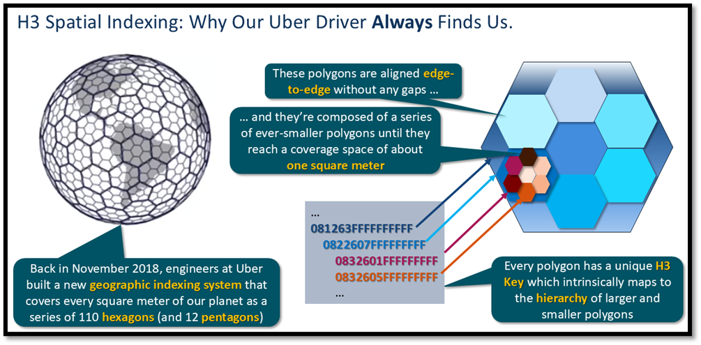
As Figure 1 shows, Uber’s solution was to develop and deploy hierarchical hexagonal indexing (H3) at the heart of its own geospatial mapping tools. Here’s a brief overview of how it works:
- Unlike the solution we saw in the prior article – a series of square tiles regressively mapped within a Mercator projection to a set of squares only a few meters on a side – H3 uses a series of polygons to more accurately cover the entire surface of the earth.
- They found that hexagons worked better than squares for mapping applications because a circle fits better within the sides of a hexagon, as well as touching the points of the hexagon. Circles are important because it’s easier to determine how many drivers are within a specific radius of a requesting rider’s location.
- One wrinkle: Because the earth isn’t a perfect sphere, H3 at its lowest resolution actually required use of 12 pentagons plus 110 hexagons for accurate coverage. (Circles still cover more area within / around a pentagon than within a square.)
- Each polygon contains a set of like polygons within it – so a hexagon encompasses seven other polygons, which in turn each contain seven other polygons, and so forth until the highest resolution level (23) is reached.
- The real elegance of this strategy is that each polygon in this hierarchical structure knows exactly which polygon is its parent in the level above it (unless it’s at lowest resolution), which polygons are its siblings at the same resolution level, and which polygons are its children (unless it’s at the highest resolution).
Corralling Data Within H3 Indexed Boundaries
In the example query in Figure 2 (below), I used the SDO_UTIL.H3_KEY and SDO_UTIL.H3_BOUNDARY functions to return the corresponding H3_KEY and H3_BOUNDARY values based on longitude/latitude pair values at a specific resolution for the photovoltaic array data stored in table EXISTING_PV_SITES.
|
1 2 3 4 5 6 7 8 9 10 11 12 13 14 15 16 17 18 19 20 21 22 23 |
WITH h3_values AS ( SELECT usgs_case_id AS case_id , state_abbr , county , pv_array_area , facility_capacity_dc , facility_capacity_ac , SDO_UTIL.H3_KEY(longitude, latitude, :res) AS h3key FROM existing_pv_sites) SELECT h3key , case_id , state_abbr , county , pv_array_area , facility_capacity_dc , facility_capacity_ac , SDO_UTIL.H3_BOUNDARY(h3key) AS h3geom FROM h3_values WHERE state_abbr = ‘WI’ FETCH FIRST 10 ROWS ONLY ; |
Figure 2: Using H3 Index Values in Simple Queries
Here’s what the query returned at resolution level 3 (Figure 3).
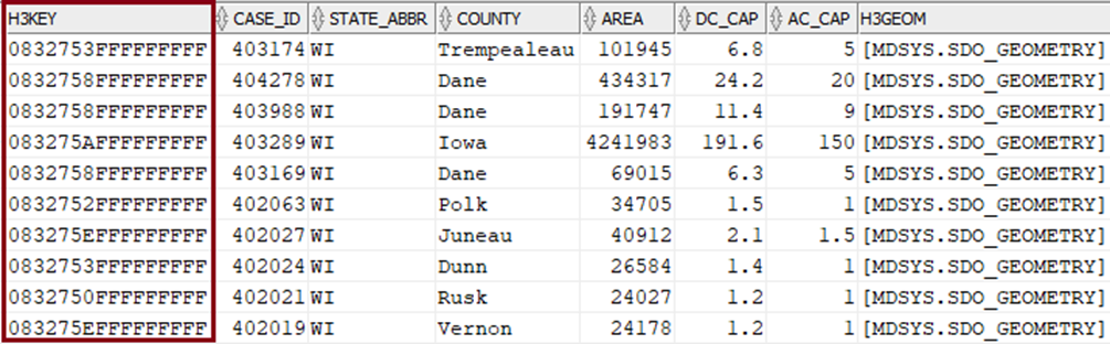
There’s a subtle difference when we compare what’s returned when the same query runs at resolution level 5 (Figure 4): the H3_KEY value for the same row is different because it represents a higher resolution.
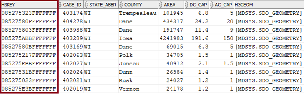
Taking a look at the corresponding boundaries that correspond to an H3_KEY value, it becomes even clearer: It’s a hexagon with its six corners defined as specific longitude and latitude pairs. For example, Figure 5 shows the contents of the SDO_GEOMETRY column for H3_KEY value 085275323FFFFFFFF from the query results in Figure 4.
|
1 2 3 4 5 6 7 8 9 10 |
MDSYS.SDO_GEOMETRY(2003, 4326, NULL, MDSYS.SDO_ELEM_INFO_ARRAY(1, 1003, 1), MDSYS.SDO_ORDINATE_ARRAY( -91.4076865340508, 44.3821017830468, -91.4955798265095, 44.3196700364542, -91.4583287104107, 44.2339873687158, -91.3335337928282, 44.2106053298784, -91.2455839698387, 44.2728414450628, -91.2824847052138, 44.3586550517715, -91.4076865340508, 44.3821017830468)) |
Figure 5: H3_BOUNDARY Values of a Specific H3_KEY Polygon
Grouping Disparate Data within H3 Indexed Boundaries
Another neat thing about H3_KEY values: Since they reference identical polygon boundaries (either pentagon or hexagon) at a particular resolution level, I can group aggregate data from multiple data sources at multiple resolution levels to provide hierarchical reporting for disparate data.
The query in Figure 6 shows exactly this strategy by first summarizing values within their derived H3_KEY for solar arrays and wind turbines at the same resolution level, then linking those aggregate values based on their matching H3_KEY attributes (i.e. within the same H3 boundary polygon).
|
1 2 3 4 5 6 7 8 9 10 11 12 13 14 15 16 17 18 19 20 21 22 23 24 25 26 27 28 29 30 31 32 33 34 |
WITH pv AS ( SELECT SDO_UTIL.H3_KEY(longitude, latitude, 5) AS h3key , state_abbr , county , COUNT(usgs_case_id) AS cnt_pv , SUM(pv_array_area) AS tot_pv_area , SUM(facility_capacity_ac) AS tot_pv_cap_ac , SUM(facility_capacity_dc) AS tot_pv_cap_dc FROM existing_pv_sites GROUP BY h3key, state_abbr, county ORDER BY h3key) ,wt AS ( SELECT SDO_UTIL.H3_KEY(geometry, 5) AS h3key , COUNT(usgs_case_id) AS cnt_wt , SUM(turbine_capacity) AS tot_wt_cap FROM existing_wind_turbines GROUP BY h3key ORDER BY h3key) SELECT pv.h3key , pv.state_abbr , pv.county , pv.cnt_pv , pv.tot_pv_area , pv.tot_pv_cap_ac , pv.tot_pv_cap_dc , wt.cnt_wt , wt.tot_wt_cap FROM pv, wt WHERE pv.h3key = wt.h3key ORDER BY pv.h3key, pv.state_abbr, pv.county; |
Figure 6: Gathering Aggregate Data from Disparate Data Sources through Matching H3_KEY Values
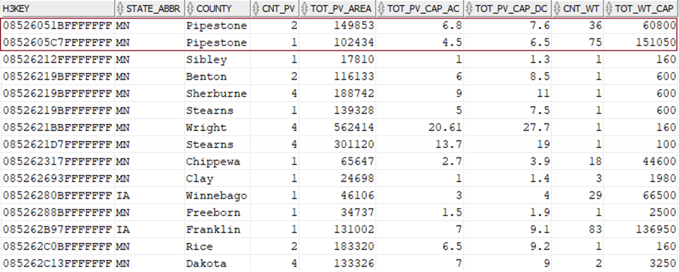
The resulting report (Figure 7) shows aggregated data from both sources, aggregated within the H3_KEY level at resolution level 5. Of course, I could also make the resolution level a query bind variable, and that would let me aggregate disparate data at that specific resolution within the polygon boundaries returned.
Using H3 Indexing Features in Mapping Applications
To leverage H3 indexing in a mapping application, I used SDO_UTIL procedure H3SUM_CREATE_TABLE to aggregate statistics related to H3 polygons into a single table.
The code in Figure 8 creates an H3 table named H3SUM_WIND_TURBINES from table EXISTING_WIND_TURBINES. I’m using that table as the data source because it has the highest number of disparate geospatial points spread out across the United States, so it’ll make mapping the aggregated data a bit more interesting.
|
1 2 3 4 5 6 7 8 9 10 11 12 13 |
DROP TABLE IF EXISTS h3sum_wind_turbines; DELETE FROM user_sdo_geom_metadata WHERE table_name = 'H3SUM_WIND_TURBINES'; BEGIN SDO_UTIL.H3SUM_CREATE_TABLE( table_out => 'H3SUM_WIND_TURBINES' , table_in => 'EXISTING_WIND_TURBINES' , geomcol_spec => 'GEOMETRY' , col_spec => '1,CNT’ , max_h3_level => 7 ); END; / |
Figure 8: Creating an H3 Table from Existing SDO_GEOMETRY Data
A few key points about how this H3 summary table was constructed:
- It will contain a simple count of the number of turbines within each aggregate
H3KEYresolution level, as the query in Figure 9 shows. - It will also contain
SDO_GEOMETRYcolumn aptly namedKEYthat describes the polygon containing the point cloud at that resolution. - Since individual wind turbines are still relatively sparse across a geography as vast as the USA, I’ve constrained the maximum H3 resolution to level 7 to limit the creation of polygons beyond that level.
- The command to delete from
USER_SDO_GEOM_METADATAsimply removes the H3 index that gets created automatically whenever an H3 summary table is created.
|
1 2 3 4 5 6 7 8 9 10 11 12 13 14 15 |
SELECT levelnum, COUNT(*) FROM h3sum_wind_turbines GROUP BY levelnum ORDER BY levelnum; LEVELNUM COUNT(*) ---------- ---------- 0 10 1 34 2 107 3 341 4 844 5 1908 6 4853 7 15709 |
Figure 9: Querying H3 Summary Table Contents
Just as I did in the prior article, I’ll transform the vector tiles that get produced from H3 Indexed data into something that mapping software can display using Oracle’s ORDS REST API toolset.
Figure 10 shows how I built an ORDS REST API module named wt_summary, defined a corresponding template that accepts variable values, and finally defined a handler that returns just the required appropriate vector tiles as a BLOB based on the parameter values specified.
|
1 2 3 4 5 6 7 8 9 10 11 12 13 14 15 16 17 18 19 20 21 22 23 24 25 26 27 28 29 30 31 32 33 34 35 36 37 38 39 40 41 42 43 44 45 46 47 48 49 50 51 52 53 54 55 |
BEGIN ORDS.DELETE_MODULE('wt_summary'); END; / BEGIN ORDS.DEFINE_MODULE( P_MODULE_NAME => 'wt_summary', P_BASE_PATH => '/wt_summary/', P_ITEMS_PER_PAGE => 25, P_STATUS => 'PUBLISHED', P_COMMENTS => 'Wind Turbine H3 Summary Tiling REST API' ); COMMIT; END; / BEGIN ORDS.DEFINE_TEMPLATE( P_MODULE_NAME => 'wt_summary', P_PATTERN => 'vt/:z/:x/:y', P_PRIORITY => 0, P_ETAG_TYPE => 'HASH', P_COMMENTS => 'Wind Turbine H3 Summary Tiling Template' ); COMMIT; END; / BEGIN ORDS.DEFINE_HANDLER( P_MODULE_NAME => 'wt_summary' ,P_PATTERN => 'vt/:z/:x/:y' ,P_METHOD => 'GET' ,P_SOURCE_TYPE => ORDS.SOURCE_TYPE_MEDIA ,P_SOURCE => 'SELECT ''application/vnd.mapbox-vector-tile'' as mediatype ,SDO_UTIL.H3SUM_VECTORTILE( H3_TABLE => ''H3SUM_WIND_TURBINES'' ,LEVELNUM => CASE WHEN z.z <= 5 THEN z*1 WHEN z.z BETWEEN 6 AND 9 THEN z-1 WHEN z.z BETWEEN 10 AND 13 THEN z-2 WHEN z.z BETWEEN 12 AND 16 THEN z-3 WHEN z.z BETWEEN 14 AND 19 THEN z-4 WHEN z.z > 20 THEN 15 END ,TILE_X => :x ,TILE_Y => :y ,TILE_ZOOM => z) as VT FROM (SELECT :z AS z) z'); END; / |
Figure 10: ORDS REST API Module, Template, and Handler for EXISTING_WIND_TURBINES Vector Tiles
This ORDS module, template, and handler are nearly identical to the examples I provided for vector tiles in the prior article, but there’s one interesting wrinkle for the zoom level bind variable (:z). Since H3 resolution is more fine-grained than vector tiles created via the GET_VECTORTILE procedure, the CASE statement in the ORDS handler ratchets up the zoom level appropriately to a slightly higher value. Otherwise, the polygons returned from the H3SUM_VECTORTILE procedure would be so small they’d be unlikely to contain any points.
Displaying H3 Summary Vector Tiles Via MapLibre GL
Since the H3SUM_VECTORTILE procedure returns vector tiles, I can reuse the majority of my code base I had already built to display them using MapLibre GL. I’ve retained the same settings for initial map position, initial zoom level and base map style; the only modifications I needed to make accommodate the wt_summary ORDS API module. Figure 11 shows the main differences:
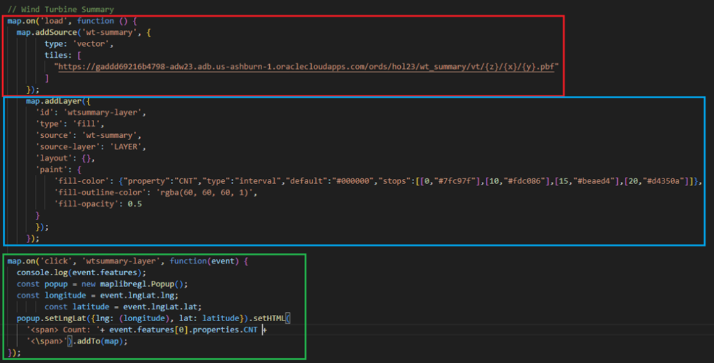
- The code in the red box accesses the ORDS endpoint for the existing wind turbines I created in Figure 11. Just as before, it connects with the MapLibreGL interface to move the display to selected vector tile contents at the corresponding zoom level for the corresponding X and Y coordinates.
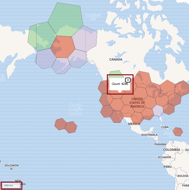
- The code in the blue box adds the layer to the MapLibreGL map. I tweaked the code here a bit to display a different color for polygons based on the total count of points captured within each polygon, ranging from light green for less than 10 points, yellow for 10-14 points, purple for 15-19 points, and red for 20 points or more.
- The code in the green box displays a pop-up when one of the polygons is clicked; it contains just the count of points captured within the polygon, since that’s the only aggregate data returned for H3 summary vector tiles.
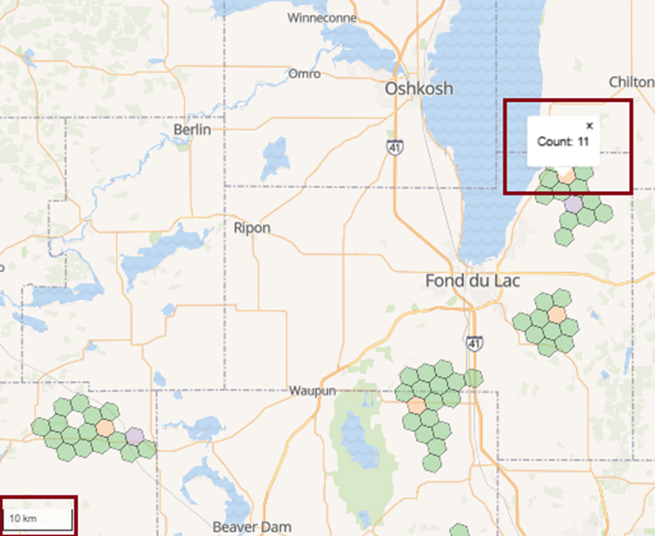
And what do the corresponding maps look like? Let’s start at nearly the lowest display level of 10 km resolution (Figure 12), which shows concentrations of wind turbines in south-central Wisconsin in the USA. Note the yellow polygon contains 11 wind turbines, providing a visual clue that area has a higher concentration than the other light-green polygons nearby:
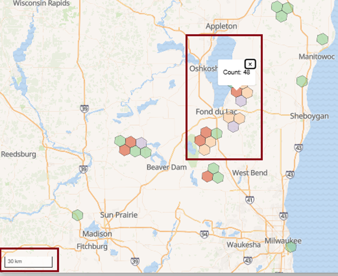
Zooming out to 30km resolution (Figure 13), the color coding of the polygons starts to make a bit more sense. Even with fewer polygons, we’re still able to identify different concentrations of wind turbines. Note the pop-up for the red polygon reflects the higher number within (48) than others nearby:
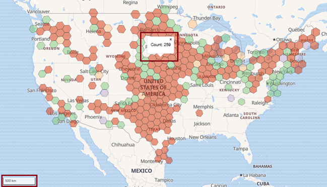
What does the view at a nearly-continental resolution level look like? At 500km (Figure 14), it’s easy to see the Great Plains of the United States is clearly the champion of wind generation for the country:
And finally, at 1000km resolution (Figure 15), we’re able to view the data from the minimum zoom level:
Vector Tile Caching
While vector tiles are easily and speedily generated in the examples I’ve presented, what about a scenario with much larger point clouds? For example, imagine a scenario for a financial institution tracking hundreds of thousands of bank branches or automated teller machines (ATMs) around the world.
If I could retain the vector tiles generated for the most commonly accessed points, that could save an enormous amount of compute time whenever a mapping application needed to display the tiles containing those points.
The good news is it’s easy to enable vector tile caching with a few simple calls to SDO_UTIL procedures. Figure 16 shows how I enabled caching for the GEOMETRY column in tables EXISTING_EV_CHARGERS and EXISTING_PV_SITES with the ENABLE_VECTORTILE_CACHE procedure:
|
1 2 3 4 5 6 7 8 9 10 11 12 13 14 15 16 17 18 19 20 |
BEGIN -- Enable vector tile caching for the GEOMETRY column in EXISTING_EV_CHARGERS SDO_UTIL.ENABLE_VECTORTILE_CACHE( table_name => 'EXISTING_EV_CHARGERS' , geom_col_name => 'GEOMETRY' , ts_name => 'DATA' , min_zoom => 0 , max_zoom => 23 ); -- Enable vector tile caching for the GEOMETRY column in EXISTING_PV_SITES SDO_UTIL.ENABLE_VECTORTILE_CACHE( table_name => 'EXISTING_PV_SITES' , geom_col_name => 'GEOMETRY' , ts_name => 'DATA' , min_zoom => 0 , max_zoom => 15 ); END; / |
Figure 16: Enabling Vector Tile Caching at Different Zoom Levels
A few points to consider from this example:
- Since there are considerably fewer solar array sites than EV chargers, I’ve stopped their caching at zoom level 15; any vector tiles at levels 16-23 would not be cached.
- Since EV chargers would likely be searched for at deeper zoom levels, I’m permitting them to be cached at the maximum zoom level (23).
- If there was an additional column of datatype
SDO_GEOMETRYin either table, it would not be cached unless specifically mentioned.
Once vector tile caching is enabled, I can query view SDO_VECTOR_TILE_CACHE$INFO to view which tables containing which columns of data type SDO_GEOMETRY are enabled for vector tile caching (Figure 17):
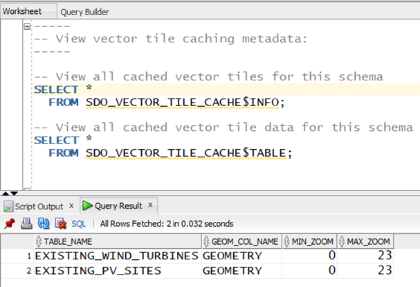
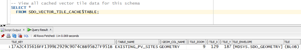
Figure 18 shows that vector tile caching is actually happening. A simple query against the SDO_VECTOR_TILE_CACHE$TABLE view shows which vector tiles have been cached as a result of queries for one or more specific vector tiles – in this case, the tile located at (X,Y) = (129,187) at zoom level 9:
Controlling Access to Cached Vector Tiles
I also have the power to limit which user accounts are allowed to leverage cached vector tiles. The code blocks in Figure 19 show two examples of access control for vector tiles:
|
1 2 3 4 5 6 7 8 9 10 11 |
BEGIN SDO_UTIL.GRANT_VECTORTILE_CACHE( schema_name => 'GEOSWARM' , read_only => TRUE ); END; / BEGIN SDO_UTIL.REVOKE_VECTORTILE_CACHE(schema_name => 'HRADM'); END; |
Figure 19: GRANTing or REVOKing Access to Existing Vector Tile Caches
- The first code block grants the
GEOSWARMuser account access to all vector tile caches owned by the executing schema via procedure viaSDO_UTIL.GRANT_VECTORTILE_CACHE. - The second code block does the opposite: it revokes access to any vector tiles owned by the executing schema to the
HRADMuser account.
Deactivating and Purging Vector Tile Caching
Finally, I have the power to deactivate vector tile caching and even purge cached vector tiles, as shown in Figure 20:
|
1 2 3 4 5 6 7 8 9 10 11 12 |
BEGIN SDO_UTIL.DISABLE_VECTORTILE_CACHE( table_name => 'EXISTING_WIND_TURBINES' , geom_col_name => 'GEOMETRY' ); END; / BEGIN SDO_UTIL.PURGE_VECTORTILE_CACHE(table_name => 'EXISTING_WIND_TURBINES'); END; / |
Figure 20: Disabling Caching and Purging Already-Cached Vector Tiles
- In the first code block, I disable vector tile caching for specific
SDO_GEOMETRYdatatype columns that could be used to generate vector tiles viaSDO_UTIL.DISABLE_VECTORTILE_CACHE. Note that if theEXISTING_WIND_TURBINEStable had anotherSDO_GEOMETRYcolumn already being cached for that table, those vector tiles would remain cached. - Likewise, as the second code block shows, I can purge any cached vector tiles for a specific table via
SDO_UTIL.PURGE_VECTORTILE_CACHE.
|
1 2 3 4 5 6 7 8 9 10 11 12 |
BEGIN SDO_UTIL.DISABLE_VECTORTILE_CACHE( table_name => 'EXISTING_WIND_TURBINES' , geom_col_name => 'GEOMETRY' ); END; / BEGIN SDO_UTIL.PURGE_VECTORTILE_CACHE(table_name => 'EXISTING_WIND_TURBINES'); END; / |
Figure 20: Disabling Caching and Purging Already-Cached Vector Tiles
Final Thoughts
I hope these two articles have enlightened you on the new mapping capabilities that Oracle Database 23ai presents, especially if you’re contemplating the deployment of an advanced geospatial solution.
The flexibility and rapid retrieval they offer should make a compelling case for leveraging your existing Oracle Database licensing as your go-to data platform before considering the adoption of other specialized geospatial databases.
Download the code featured in this article
If you’d like to experiment with the APEX 24.2 app and the MapBox examples to explore the mapping features presented in this article, you can download all application code samples here.

FAQs: Building High-Performance Maps with Vector Tiles and H3 Indexing
1. What are vector tiles and why are they important for map performance?
2. How does the H3 index improve spatial queries?
3. Why combine 23AI vector tiles with H3 indexing?
4. Can these techniques be used with open-source tools?
5. What are the main benefits for developers?
Subscribe to the Simple Talk newsletter
This document contains proprietary information and is protected by copyright law.
Copyright © 2026 Red Gate Software Limited. All rights reserved


Load comments