Creating Uber-Fast Maps With 23ai Vector Tiles and H3 Indexes: Part 1

Oracle Database 23ai added 300+ new features like the new VECTOR datatype that get most of the attention, but often overlooked are two new features that dramatically expand support for complex geospatial problem-solving. In this article we’ll take a closer look at vector tiling – a toolset that already has everything your developers need to create ultra-fast maps in standard geospatial applications.

OK, I have to admit it: I’m a map junkie. I’ve built all kinds of mapping applications for the past several years using either Oracle APEX’s Native Map Region (NMR) toolset when I wanted a low-code solution with excellent control over features like legends and layers, and Oracle Spatial Studio when I didn’t have time to write complex SQL to quickly review how spatial data was distributed.

One pain point I’ve run into involves response time, especially when I’m displaying tens or even hundreds of thousands of individual points on a map on different layers. Even my laptop with a reasonably robust GPU and memory cannot cope with those demands. For example, the map in Figure 1 was built in APEX 24.2 using NMR to display over 157,000 separate longitude/latitude points on three different map layers, and it typically takes between 45 – 180 seconds to load completely. My pain is not new or just my pain; loading map content quickly when there are huge volumes of individual points to display has been a challenge for GIS applications since they were first born in the mid-1960s.

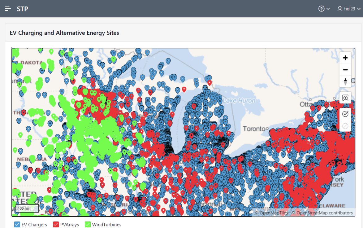
Figure 1. Displaying +157K Distinct Geographic Points in Oracle APEX 24.2

But there’s good news for Oracle developers working with geospatial applications today: There’s an intriguing solution in Oracle Database 23ai that significantly reduces map response time. Vector tiles encode all mapping data – both point / polygonal information and corresponding metadata – into a unique compressed binary format so specialized GIS applications like QGIS or MapLink can interpret and display this format at blinding speed.

Since the size of the data for vector tiles is dramatically smaller than previous formats, network response time is also reduced, so ultimately response time for any map activity – scrolling, zooming, or selecting individual points and displaying their metadata – often improves by several orders of magnitude.

So, What Are Vector Tiles?

The easiest way to envision vector tiles is to imagine a Mercator map projection of the surface of the Earth. The resulting projection of that geometry onto a flat surface results in a series of evenly-sized squares that can be grouped into just four at the lowest zoom level (Figure 2).

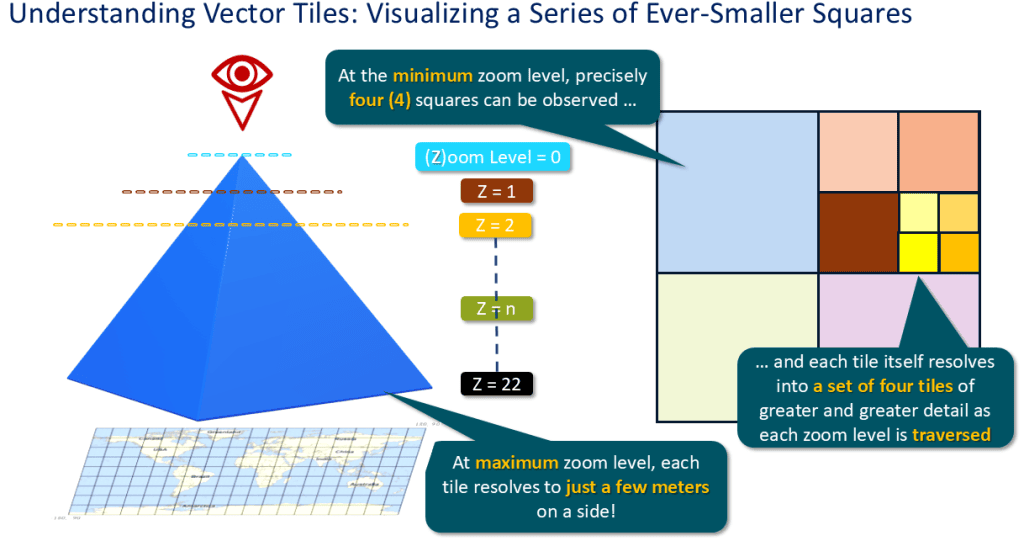
Figure 2. Vector Tiles: Grouping Ever-Lower Levels of Mercator Projection Squares

Here’s the real brilliance of vector tiles: At the next lowest zoom level, each one of those four squares also contains another set of four squares, which at the next zoom level contains yet another four squares, and so on until we reach a zoom level of 22, or 2²³ squares. At this lowest level, each vector tile is a square that’s just under one square meter in area.

Vector tiles work really well for mapping applications because at a high zoom level, it’s easy to see where points are concentrated on a map, and as you drill down into the lowest levels of the map, the points are already present so there’s no need to make another round trip to the map server to retrieve them and any related metadata.

Vector Tiles: Preparing For Implementation

Let’s illustrate how easy it is to leverage 23ai’s vector tile capabilities with a straightforward use case: A public utility is researching where it should place long-term battery storage sites close enough to existing wind turbines, solar panel farms, and other renewable energy resources it’s planning to develop. Since EVs aren’t going to disappear and are likely to increase among its customer base, the utility also needs to identify all existing EV charging stations so they can provide them with energy captured at the battery storage sites.

To build out this use case, I’ve created and populated three different tables containing geolocations for EV charging stations, wind turbines, and photovoltaic (PV) solar panel farms throughout the United States. These data were downloaded and curated from the US National Renewal Energy Laboratory (NREL) website, and contains site-specific information including each wind turbine’s latitude and longitude.

Note: in the Appendix at the end of this article, you can find details about how to get the structures and data to test this out yourself.

To keep this example simpler for now, I’ll focus on the EXISTING_WIND_TURBINES table. The DDL to create that table is shown in Figure 3.

Figure 3. EXISTING_WIND_TURBINES Table Creation

After uploading the data via the SQL Web Developer data loading facility, I updated the contents of the GEOMETRY column with the longitude and latitude of every wind turbine site. Finally, I created a spatial index on each table’s GEOMETRY column (Figure 4), thus enabling the geospatial features of the SDO_GEOMETRY datatype so that mapping technology could interact with that column’s data.

Figure 4. Updating EXISTING_WIND_TURBINES.GEOMETRY and Creating Its Spatial Index

Building Vector Tile Output From an SDO_GEOMETRY Column

Returning geospatial data from the EXISTING_WIND_TURBINES table as a series of vector tiles in binary format is remarkably simple to accomplish via the new 23ai SDO_UTIL.GET_VECTORTILE function. Note that in this case, I specified the exact zoom level and X and Y coordinates of the tiles I’m interested in retrieving (Figure 5), but we’ll look at parameterizing this function call shortly.

Figure 5. Generating Limited Vector Tile Output from EXISTING_WIND_TURBINES

So what gets returned from the query in Figure 5? Here’s a snippet of the resulting output (Figure 6); you’ll note it appears as gibberish on first glance. However, a spatial application that consumes this output sees this binary output as tightly-compressed spatial data comprising the vector tiles themselves as well as any specific metadata about each point. The spatial application can then display the vector tiles within a separate mapping layer at extreme speed without the need to make a return trip to the sending server.

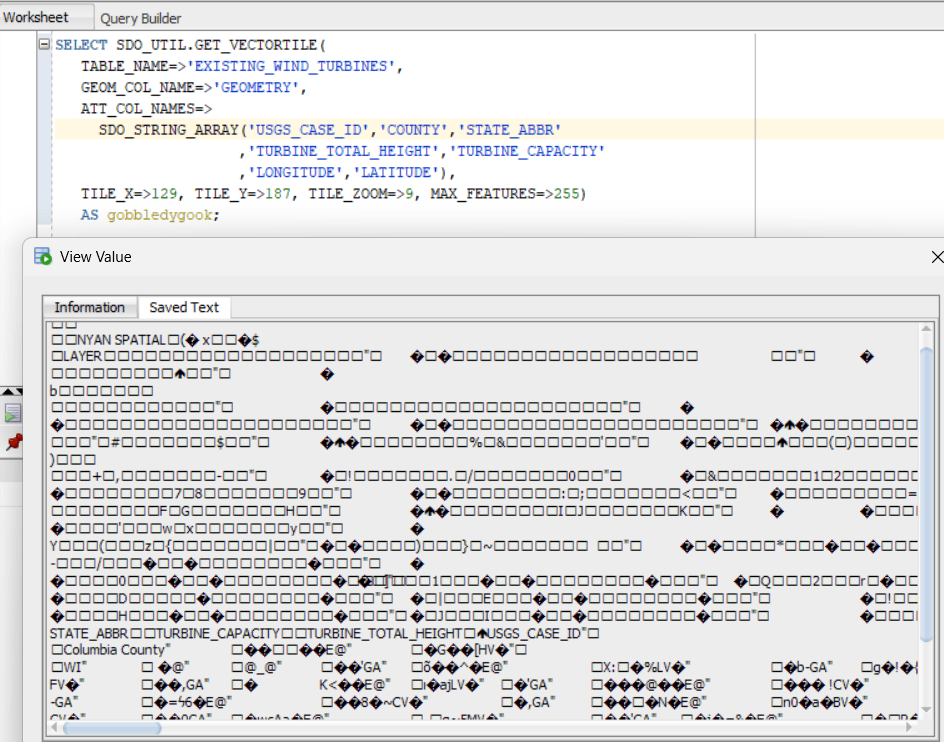
Figure 6. GET_VECTORTILE Function: Sample Output

Generating Vector Tiles Via ORDS REST API

The trick to transforming these vector tiles into something that mapping software can use to display them is leveraging Oracle’s ORDS REST API toolset. Figure 7 shows how I built an ORDS REST API module named wind_turbines, defined a corresponding template that accepts variable values, and finally defined a handler that returns just the required appropriate vector tiles as a BLOB based on the parameter values specified.

Figure 7. ORDS REST API Module, Template, and Handler for EXISTING_WIND_TURBINES Vector Tiles

The ORDS module and template code is pretty simple, but the ORDS handler code is a bit trickier to understand, so let’s take a closer look:

The query also expects three bind variable values to be supplied during execution:

Enabling Vector Tile Displays with MapLibre GL

While I could use Oracle Spatial Studio to map vector tiles, it takes some extra time to configure a user account and set up all the metadata and infrastructure to leverage that powerful toolset. Here’s a slightly faster method I can use as a touchstone to verify that I’ve set up my Oracle 23ai database-side code properly for mapping purposes with easy-to-understand HTML:

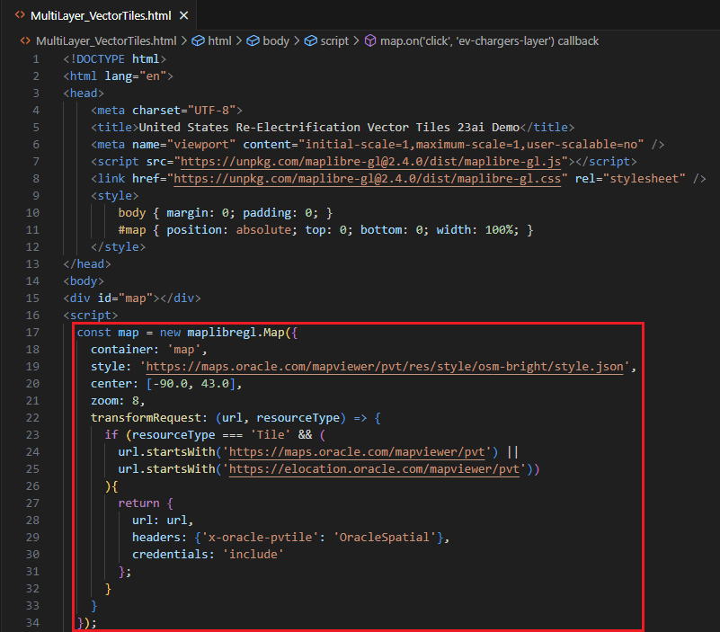
Figure 8. MapLibre Live Server Demonstration: Initialization & Setup

The rest of the HTML body is where the real magic of vector tiles shines through. In Figure 8, I’ve highlighted the code that builds that handles mapping all of the existing wind turbine points:

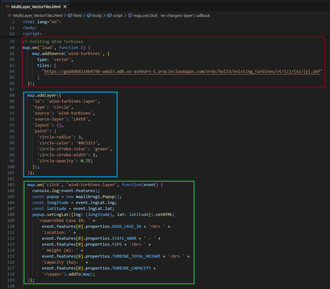
Figure 9. MapLibre Live Server Demonstration: Adding a Map Layer

The End Result? Blazingly Fast Map Displays.

As much as I love using APEX Native Map Regions, I was thrilled to see that displaying map points with vector tiles and MapLibreGL is at least an order of magnitude faster … and I’m running my tests on a low-cost, underpowered ASUS VivoBook laptop without any display accelerators or GPUs. I was able to traverse, zoom in, zoom out, and navigate within the map frame with significantly less lag time.

And I saw no degradation in performance when I added two more mapping layers – existing photovoltaic arrays and existing EV charging stations – to my mapping configuration. Figure 10 shows the result, with EV chargers shown in blue and PV arrays shown in red within the continental the United States.

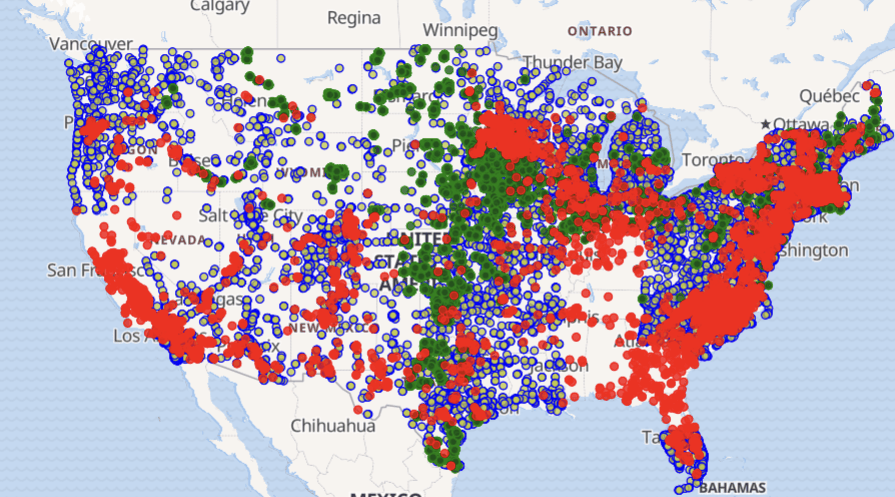
Figure10. Vector Tile Maps: Wide-Area Map Display

Figure 11 shows the upper Midwest of the USA at a lower zoom level. Note that individual points are still quite clearly displayed even at this zoom level.

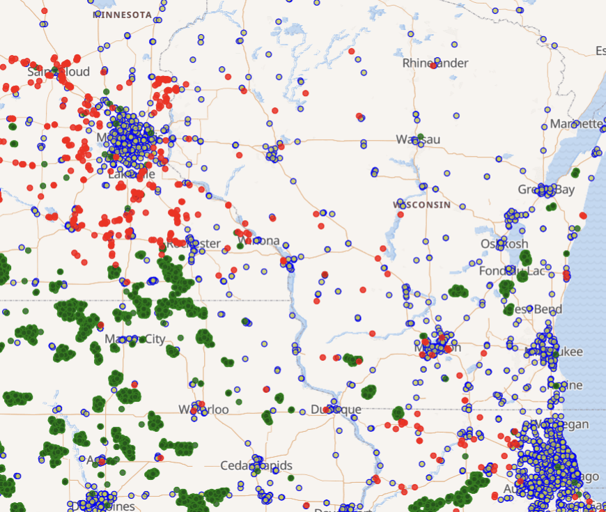
Figure 11. Vector Tile Maps: Drilling Down to Lower Levels of Detail

Finally, Figure 12 shows an example of drilling down deeply into the map and then showing some of the metadata for one of the hundreds of thousands of map points – in this case, a single wind turbine in middle of Minnesota.

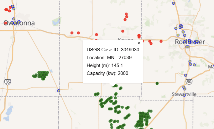
Figure 12. Vector Tile Maps: Zooming In Even Lower

Enough Tiling Already! What’s Coming Next?

Vector tiles are just half of the new mapping capabilities that the Oracle 23ai converged database provides for your IT organization’s mapping requirements. They’re relatively simple to implement if you’ve already embraced the SDO_GEOMETRY datatype for geospatial applications, and they’re also likely to rescue your DevOps team from painful experiments with different geospatial databases.

In the next article in this series, we’ll look at how Hierarchical Hexagonal Indexing (H3) features in Oracle 23ai handle another type of mapping problem: visually aggregating the data that’s often implicitly attached to hordes of individual geographic points so we can provide meaningfulness at any zoom level.

Appendix

If you’d like to experiment with the APEX 24.2 app and the MapBox examples presented to see the dramatic difference in performance, you can download all application code samples, DDL to create tables and spatial indexes, and GIS datasets themselves here.