Aggregation is a widely used way to summarize the content of a database. It is usually expressed with GROUP BY clause or just using aggregate functions (like COUNT or SUM). When the database engine executes a query with aggregations, it produces individual rows need to compute the required output and then performs the aggregation as (almost) last step. We discuss in this article how to re-write a query manually so that the order of operations will be different and when it can be beneficial.

We start with remainder that SQL is a declarative language, that is, a properly written query specifies what should be included into result but does not specify how to calculate this result. There are several ways (called execution plans) to do that for almost any query. All execution plans for a query produce same results but may utilize different amounts of computing resources. An optimizer tries to choose the best plan for execution. Usually, state-of-the-art optimizers do their job well but sometimes they fail to choose a good plan. This may happen for different reasons:

• The data statistics and/or cost model are imprecise.
• The optimizer does not consider some classes of plans.

In this article we discuss one type of query transformation that most optimizers do not use. Because of this, it can be beneficial for you to rewrite a query to help the optimizer order operations in a way that can be beneficial.

An analytical query is supposed to produce some kind of summary generalizing properties of huge amounts of data but at the same time should be compact and easy for humans to understand. In terms of the SQL query language this means that any analytical query extracts and combines large number of rows and then uses aggregate functions with or even without GROUP BY clause. More specifically, we consider queries that contain many JOIN operations followed by aggregation. Usually, queries are written in this way and, surprisingly, the optimizers choose the best order of joins but leave the aggregation as the last step.

Aggregation reduces the number of rows that will eventually be output from the query. Intuitively we can expect that it is possible to reduce the quantity of resources needed for execution if aggregates could be computed before joins. Of course, this is not always possible (for example when the argument of an aggregate function combines columns from joined tables), but even partial aggregation can reduce the cost significantly.

Our example uses the postgres_air database which can be downloaded from (https://github.com/hettie-d/postgres_air). You can download and restore the database if you want to execute any of the code in the article yourself.

The following ER diagram shows a subset of the tables in the postgres_air database that are important for our example. The tables that will be used in the example query are highlighted with the green background.

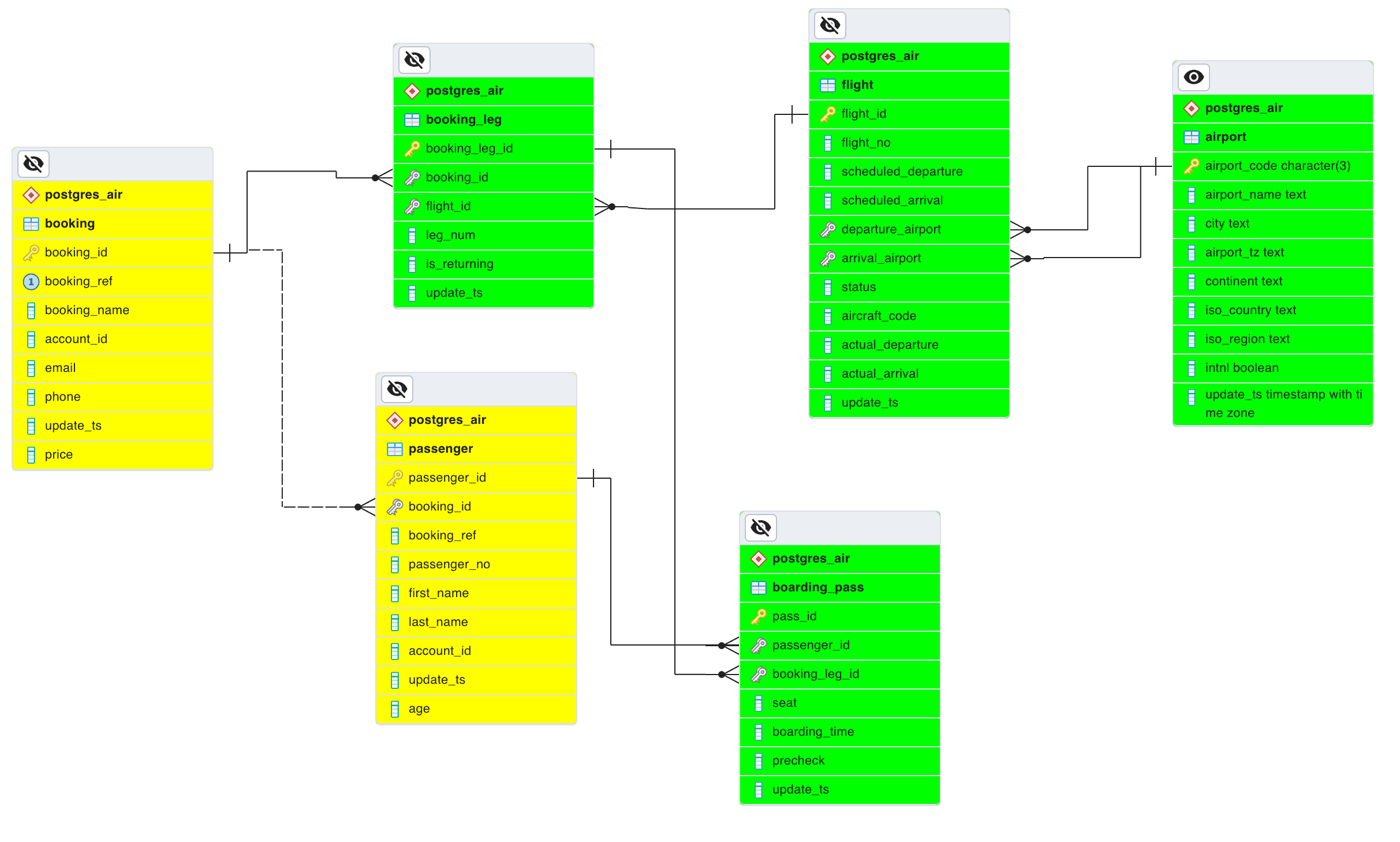
A row in the table booking represents a ticket. Each ticket is for one or more passengers and is linked to one or more flights. The table booking_leg is actually a relationship between the booking and flight tables. We do not need the booking and passenger tables in this example. A boarding pass is issued for each passenger, for each leg in the booking. We use a modified query discussed in [1, chapter 6]. The query returns the number of passengers departing from an airport during a month. To make results compact, the query returns5 airport-months with largest numbers of passengers:

The limit of the output to 5 rows does not significantly affect the execution time because the rows are sorted and, therefore, all rows must be produced.

When SQL query performance is discussed, the best place for a DBA to start is with analysis of the execution plan. So, the execution plans are included below. However, if you are not comfortable reading large execution plans but know or can believe that time needed for execution of a query depends mostly on the size of tables, you can skip the execution plan and go to a compact summary after the execution plan.

Even without any analysis we can guess that the number of boarding passes is significantly larger than the number of airports. This observation can be confirmed with an execution plan:

The following table presents the essential data in more compact form:

Table or table expression	Number of rows
airport	692
flight	683178
booking_leg	17893566
boarding_pass	25293491
All tables joined	25293491
After GROUP BY	2568
Booking_les with boarding_pass	8841899
Booking_leg join boarding_pass group by flight_id	254253

Each boarding pass row is counted exactly once, therefore, the number of rows after all joins is equal to the number of boarding passes. Boarding passes are issued not earlier than 24 hours before the departure. Therefore, there are no boarding passes for future bookings. For the same reason, the number of flights in the last row of the table is less than the total number of flights.

These observations suggest that we can try to reduce the number of rows after joining the two largest tables, namely, booking_leg and boarding_pass. The modified query looks somewhat more complicated but the execution time is significantly better:

Note that the intermediate grouping in this query is partial: it counts passengers on each flight but final grouping is still needed. The query returns exactly the same rows as the original one, but the execution time is below 12 seconds, while the original query took almost 24 seconds. This can be confirmed with the execution plan below (again, you can skip it if the difference in the execution time already convinced you):

Any experienced DBA will notice that our execution plans do not contain enough information describing input/output needed for the query execution (such as number of buffers). There are two reasons for that:

• Both plans contain hash joins only, so each row of input tables is accessed only once for both queries and I/O is exactly same.
• Our queries are CPU-bounded, rather than I/O-bounded. There is no need to store any intermediate results between operations, and even sort uses main memory only.

So, is this kind of query transformations beneficial?

The answer is: it depends. Looking at the plan, if you compare the number of rows accessed to output the result, it is exactly as it was in the previous example. But the total costs were quite different:

Original query:

(cost=8513712.70..8513712.73 rows=5 width=49)

Rewritten query:

(cost=3148532.58..3148532.61 rows=5 width=73)

In the database folklore the JOIN operation is considered as a major resource consumer. However, the aggregation (grouping) has approximately same complexity as a join. This transformation includes additional grouping of a large table (or large intermediate result) in a hope to reduce complexity of subsequent join operations.

In our example the transformation reduces the number of rows from approximately 25 millions to 250 thousands. This reduction dramatically reduces the time needed for subsequent operations.

Transformation Rules

We are now ready to define the transformation rules. The query suitable for the transformation should contain joins followed by an aggregation (either GROUP BY or just returning one row), and the arguments of the aggregate functions must depend on a subset of joined tables. The code below is pseudocode, please do not try to execute it. We represent such queries in the following generic form:

The result of the transformation of this generic query is:

Informally, the transformation introduces additional grouping before the join. Aggregate functions needed after transformation may differ from the function in the original query (we discuss that later). Both table_a and table_b can be table expressions. Grouping and joining may involve multiple columns.

The table below shows how the example query from the previous section can be derived from the general form.

Aggregate Function	COUNT (attributes)
table_b_attrib	passenger_id
table_a	flight JOIN airport
table_b	booking_leg JOIN boarding_pass
join_attrib_a	flight_id
join_attrib_b	flight_id
gr_attrib_a	city, f.departure_airport,month
gr_attrib_b	– – EMPTY – – –

What about aggregate functions?

The example in the previous section uses COUNT as an aggregate function. In this section we provide transformation rules for other SQL aggregate functions.

We have already seen that for count in the original query agg_func1=sum and agg_func2=count. Functions SUM, MAX, and MIN are easy: agg_func1=agg_func2=agg_func for these functions. Indeed, these functions are commutative and associative. Therefore, arguments can be grouped arbitrarily in any order. The same applies also to the following aggregate functions available in PostgreSQL: bit_and, bit_or, bit_xor, bool_and, bool_or text.

The function AVG is trickier. By definition, the average is a ratio of sum of values to the quantity of these values, so the subquery can compute SUM and COUNT separately, and the final aggregation should divide sum of values by the sum of counts. However, the aggregate function sum ignores NULL values, while count(*) does not. Therefore, the correct expression should use count(column_in_sum). Also, the value of sum must be converted to float or double type before division.

An aggregate function that returns a concatenation of its input (such as string_agg, array_agg, xel_agg) depends on the order of rows and therefore cannot be used together with eager aggregation.

Yet another complication is the keyword DISTINCT that can precede the argument of any standard aggregate function. Again, functions max and min are easy as they are idempotent: the value of max or min remains same no matter how many times this value occurs as an argument.

Functions like (distinct attr_val) and sum(distinct attr_val) require preliminary aggregation on attr_val that actually removes duplicates.

Can an Optimizer Do This?

Looks like our transformation can be defined in a pretty formal way. It is known for very long time (see, for example, [2]. Can a database optimizer do this transformation automatically?

The answer is: yes, it can, but, most likely, the optimizer of your favorite RDBMS does not do it. In this section we discuss why developers of your favorite optimizer decided not to do that.

Most optimizers use some variations of the dynamic programming algorithm known since the late 70s. This algorithm finds the best (according to the value of the cost function) order of operations for SPJ (select-project-join) queries. Actually, handling of S and P is easy, so the optimization problem is also widely known as a problem of join order selection. In other words, such optimizers accept queries containing joins only. What to do with other operations? Some optimizers just split the query on SPJ parts and optimize them separately. For example, joins before and after the aggregation are optimized separately. We cannot see that from the execution plans, because the order is the same. However, in general our transformation may force early execution of some joins that the optimizer would execute later if all joins would be optimized together.

The benefits of our transformation are conditional: the cost of additional eager aggregation must be less than the gain on subsequent join operations due to reduction of the argument size. This means an increase in computational complexity that might be undesirable.

The good news is that researchers already found efficient techniques suitable for these kinds of query transformations, including more difficult transformations for outer joins and semi-joins [3]. We did not discuss joins other than inner in this article.

So, if your optimizer does not do eager aggregation yet, you can try doing it manually. Before doing it estimate how significant the reduction of size will be and choose the right place for eager aggregation. Most likely, the query that can benefit from eager aggregation contains joins of large and small tables. All large tables should be joined before the intermediate grouping.

References

1. Henrietta Dombrovskaya, Boris Novikov, and Anna Bailliekova. Post- greSQL Query Optimization. Apress, 2021. URL: http://doi.org/10. 1007/978-1-4842-6885-8, doi:10.1007/978-1-4842-6885-8.
2. Yan,W.,Larson,P.A.:Eageraggregationandlazyaggregation.In: Proceedings of International Conference on Very Large Data Bases (VLDB), vol 95, pp. 345–357 (1995)
3. Marius Eich, Pit Fender, Guido Moerkotte: Efficient generation of query plans containing group-by, join, and groupjoin. VLDB J. 27(5): 617-641 (2018)