The series so far:

• Translating a SQL Server Schema into a Cassandra Table: Part I Problem Space and Cassandra Primary Key
• Translating a SQL Server Schema into a Cassandra Table: Part II Integrity Constraints 
• Translating a SQL Server Schema into a Cassandra Table: Part III Many-to-Many, Attribute Closure and Solution Space 

A subset of related tables in a relational schema can satisfy any number of queries known and unknown at design time. Refactoring the schema into one Cassandra table to answer a specific query, though, will (re)introduce all the data redundancies the original design had sought to avoid.

In this series, I’ll do just that. Starting from a normalized SQL Server design and statement of the Cassandra query, I’ll develop four possible solutions in both logical and physical models. To get there, though, I’ll first lay the foundation.

This initial article focuses on the Cassandra primary key. There are significant differences from those in relational systems, and I’ll cover it in some depth. Each solution (Part III) will have a different key.

Part II uses – and this may surprise you – several techniques from the relational world to gain insight into the primary key choices and their implications as well as redundancy points.

Part III employs the foundation from I and II both to design and evaluates each logical and physical model pair.

A background in relational databases and theory is essential, but not Cassandra. I’ll present enough context as the series progresses.

The Problem

The sample transactional database tracks real estate companies and their activities nationwide. Its data is growing into the terabyte range, and the decision was made to port to a NoSQL solution on Azure. The downsides are the loss of the expressive power of T-SQL, joins, procedural modules, fully ACID-compliant transactions and referential integrity, but the gains are scalability and quick read/write response over a cluster of commodity nodes.

Among the SQL Server 2017 artifacts is this greatly simplified, fully normalized four-table diagram:

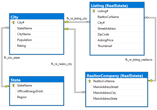
Figure 1. Normalized SQL Server schema

Both relational and Cassandra database design (should) go through conceptual, logical and physical analysis. They use the same conceptual model, mostly an ER diagram, but veer off starting at the logical design. The diagram for this purpose is an ER replacement; I’ll use it to pick attributes for what I’ll term a “unified relation,” the structure created by merging entities into one, which is to become the Cassandra table. Verifying against enterprise rules, Figure 1 is fully normalized (through 5NF). There is no redundancy.

This is the query, aka data access pattern, that the single Cassandra table is to support:

Q_k Find listings for a realtor company in a city

The resultant Cassandra table will be a denormalized, partitioned and sorted dataset on cluster nodes’ discs meant to answer the query efficiently for any given realtor company-city pair(s). More generally, as joins are not supported, a table is a precomputed result set from which data is sliced. The method is moving from organizing data around meaning to query-first design.

Answering the sample query Q_k doesn’t require all attributes, or even most, from the diagram. Many of the attributes would have been provided to the app by previous workflow access patterns or needed by later ones. I include them to show dependencies and redundancies in solutions to come.

The Cassandra Primary Key

This primer is meant to be enough to understand key designs in the solutions and a little more. A Cassandra Primary Key consists of two parts: the partition key and the clustering column list.

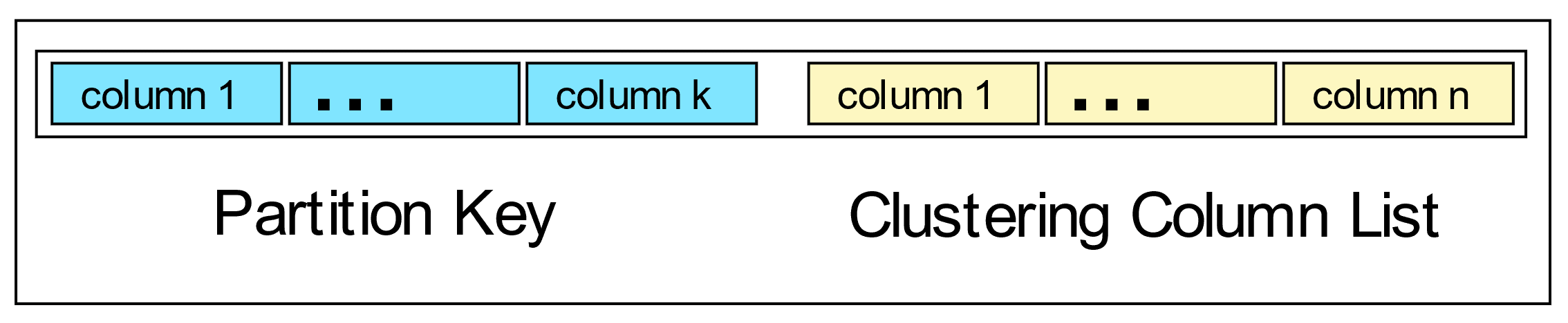
Figure 2. Two-part primary key

I’ll use this shorthand pattern to represent the primary key: ((AB)CDE). The inner parentheses enclose the partition key column(s), and clustering columns follow. In the solutions, columns in the logical and actual table primary key definitions are in the order presented. Order matters!

The design of the primary key affects data locality, sorting on disc, and performance. Keep in mind that the attributes chosen are those to be constrained in CRUD operations.

In addition, there is no notion of an alternate key and no referential integrity and so no foreign keys. Cassandra allows a limited form of indexing at times useful for retrofit queries but not meant to be used for the primary query for which the table was designed.

As with relational databases, the Cassandra primary key uniquely identifies rows. This does not mean, however, that its key patterns follow rules for unique key design in the relational model – far from it. An important deviation as you’ll see is that the key commonly combines attributes that can appear separately in unique keys and non-unique indexes. Another involves data types not available in relational systems.

Collection Data Types: Extending Key Design Possibilities

Parts II and III explore concepts demonstrated here in more depth. For now, I give a basic example of how a key can be “unique” in a non-traditional manner.

Cassandra Query Language (CQL) data types include collection types, which are not permissible in the relational model (by 1NF): list, set, map, tuple and user-defined type (UDT). A UDT groups related fields in a structure.

This graphic shows how two entities associate as per enterprise rules in the “listed by” relationship:

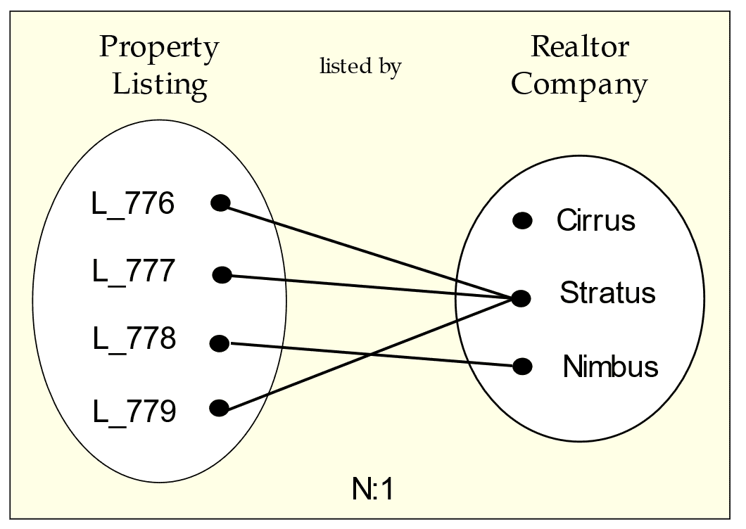
Figure 3. Occurrence diagram: many-to-one from Listing to Realtor

Say the query is this: Find the realtor for a listing. Since CQL has no joins, the listing identifier must be in the key so you can search on it, the realtor identifier and its other data should be non-key columns, and that there must be one row per listing. Specifically, the “many” side functionally determines the “one” side.

As for redundancy: this is expected in Cassandra for performance as it obviates the need for multi-pass queries. A major challenge, though, is keeping duplicated data consistent between rows (let alone between tables). Here, any data in a dependency relationship with the realtor identifier can be redundant.

Now turn the query around: Find all listings for a realtor. Realtor is placed in the key for searching, but for demonstration purposes, place listings outside the key in a set as this sample CQL written in DataStax Studio shows:

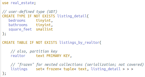
Query over two partitions – see next section – and result:

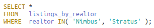
I’ve omitted a lot here. The point is this: the one-side key uniquely identifies its row but could not be a unique key in SQL Server. I generalize the concept to mean that any key column(s), used for uniqueness or not – see the section below on clustering columns – can reverse functional dependency with collection types.

A final point. Any key column can also be a collection (example later).

Partition Key

This first part of the primary key definition consists of one or more columns and divides the table’s rows into disjoint sets of related rows. The partition also is the atomic unit of storage – its rows cannot be split among nodes – and so column choice is important to physical design size considerations as well as logical row grouping for efficient querying and modification.

Each partition of replicated rows is automatically and transparently placed on nodes in the Cassandra cluster via partition key hashing. During CRUD operations, Cassandra can instantly locate partitions without scanning the potentially large cluster.

For the initial access pattern that a table is to support, you get the best performance if you design for equality comparisons on the partition key, and if multiple columns, you constrain on each column. As an example, here is a CQL query returning all rows on two partitions given partition key columns realtor company and state, abbreviated (RS):

Inequality comparisons or failure to constrain on all partition key columns results in unpredictable (generally poor) performance. Good performance often requires that Cassandra find rows in one partition, or failing that, a very small, knowable set of partitions as does the sample.

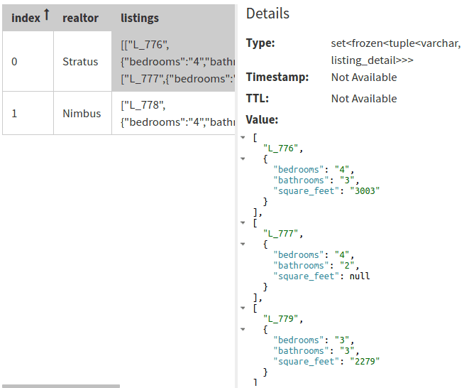
Static columns are data not repeated in each row but stored once in its partition. This is possible because any given static column is in a dependency relationship with a subset of partition columns.

As an example, let (RSC) be the partition key where “C” is city. The combination (SC) functionally determines city population, and S, the governor, state bird, flag and other attributes when known:

There is much redundancy across partitions when an (SC) or S value is repeated, but much less so than if the statics were in each row in a large partition.

There can be no static columns, however, if there are no clustering columns.

Clustering Columns

Unlike the partition key, the list of clustering columns in the primary key definition is optional. When absent, a table partition has at most one row: the partition column(s) uniquely identifies its row.

When present, clustering columns enable a partition to have multiple rows (and static columns) and establish the ordering of rows within the partition. Just as Cassandra uses the partition key to instantly locate row sets on a node(s) in the cluster, it uses the clustering columns to quickly access slices of data within the partition.

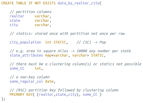
The ordering of clustering columns in the primary key definition follows this sequence:

Figure 4. Clustering column conceptual breakdown

Any subset of these clustering column types may be in the primary key clustering column list, as long as they are placed in this order. CQL, though, has no notion of these types – certainly no syntax – but it matters to the query.

In the opening section for the Cassandra primary key, I stated that the key can be a mix of attributes for uniqueness and others for searching or different ordering from non-unique indexes – Figure 4 is meant to show this. A key having any of searching or ordering attributes accompanying those for uniqueness is, in relational terms, a non-minimal superkey. Such is a near-guarantee for data corruption in relational OLTP systems, but common in the Cassandra key.

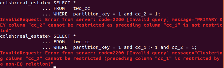
In the WHERE clause predicate, a query can filter on no clustering columns to get all rows in a partition or all of them to pinpoint one row. It can get contiguous ranges of rows off disc by constraining on a proper subset of them. CQL, however, will not allow a query to filter on a clustering column if the clustering columns defined in the list before them are not also constrained.

One more important restriction: once a clustering column in the WHERE clause is filtered with a non-equality operator, no clustering column following it in the list may be constrained.

I’ll use this table with two clustering columns to illustrate:

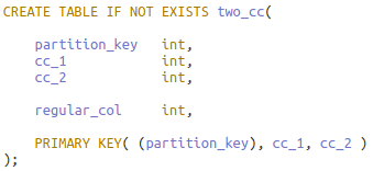
The CQL shell (CQLSH) utility show two errors in violation of the rules:

The first two types of columns shown in Figure 3 form the “search attributes.” Columns meant to be constrained on equality operators “=’ and “IN()” may be followed by columns more likely to be filtered with inequality operators such as “≤.” Queries with an inequality operation used on an equality column and conversely equality operations on inequality columns will work, subject to the above restrictions.

Ordering columns can be appended next to the clustering column list to further affect data layout on disc. It is essential to realize that ordering columns – in fact, clustering columns in general – do not order over the entire table but only within the slice of rows in the partition defined by the clustering columns in the list before them. As with previous clustering column types, a query may or not filter on these columns.

Columns in the last position, if any, are added as necessary to make the primary key unique. The assumption is that these appended columns – assuming there are clustering columns defined before them – are not critical to searching and sorting. Placement higher in the list would hamper this ability. And further, it is often the case that their values, when not constrained upon in the query, are needed in the result set. While this is recommended form, do recall the deviant case from the collection types section in which the key remains unique although the “uniqueness” columns are in an off-key structure.

Finally, another way to affect data layout is to make any clustering column ascending, the default, or descending. Logical models will show each clustering column annotated with the “C↑” or “C↓” arrows, but the actual table definitions will all have ascending columns, so their specifications are not shown.

The Combined Key

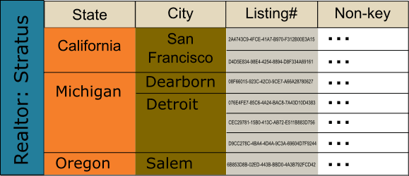
Figure 5. Conceptual row nesting in a partition

The graphic shows the nested layout for possible rows given key ((R)SCL) where abbreviations R and S and C are as before, and “L” for Listing# appended to make the key unique. The static columns for partition key R are not shown. Aside from those columns, you can visualize with a CQL query a three-row result set containing C and L and all non-key columns sliced from the partition:

Here is a summary of some properties of the primary key; compare how in each case they differ from the relational primary (or alternate) key:

• Key columns are immutable
• The key is often a non-minimal superkey
• The key may not functionally determine its rows (while remaining unique)
• Any key column may be a collection
• Key and non-key column dependencies may fail any level of normalization

As to the third point: in the collection types section, you saw the “one” side of a many-to-one relationship placed in the key and the “many” side in a set of nested collections as a non-key attribute. I illustrate the fourth by reversing this; this valid table definition uses collections for the partition and a clustering column:

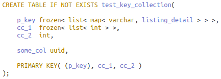
Key or not, collections fail 1NF.

During physical design, clustering columns can be moved into the partition key to create more partitions with fewer rows, or movement in the opposite direction to create fewer partitions with more rows. The decision also affects which columns become static.

In most solutions, I will use combinations of attributes ((R)SC) in the key. The final designs, though, could be based on ((RS)C) or even ((RSC)). This is noted but not considered further.

Conclusion

You’ve seen that Cassandra tables have partition columns for data locality among nodes and their attendant static columns. Clustering columns and rigid CQL query restrictions are aimed at optimizing contiguous row retrieval and processing. Every table is a denormalized, precomputed result set from which data is sliced. Tables typically have a non-minimal superkey if that. Understanding collections as key and non-key columns with little or no indexing as we’re accustomed to thinking is quite an adjustment.

Add to this the redundancy that denormalization implies; converting to a system that not only expects data duplication between rows in a single partition, across partitions and tables as well but requires it for responsiveness. Any table can fail normalization levels in multiple places via relationships involving key and non-key columns.

Cassandra does have mechanisms to keep replicated rows in sync and some ACID compliance. It has durability always, atomicity and isolation to a partial degree but nothing for all the other consistency and integrity checking we’re used to ranging from alternate and foreign keys and transaction isolation levels to stored procedures and triggers. It all implies a tight coupling with the OLTP app and the development of new apps to find integrity problems.

In Part II, I’ll continue foundation with relational analysis using tools such as occurrence and functional dependency diagrams, and a function that computes closure over a set of attributes and determines whether the set would be a superkey for the unified relation.