The series so far:

• Translating a SQL Server Schema into a Cassandra Table: Part I Problem Space and Cassandra Primary Key
• Translating a SQL Server Schema into a Cassandra Table: Part II Integrity Constraints 
• Translating a SQL Server Schema into a Cassandra Table: Part III Many-to-Many, Attribute Closure and Solution Space 

This last in the series continues with an exploration of the many-to-many relationship. Then it returns to an analysis by functional dependency with attribute closure which is important in establishing “uniqueness” in the Cassandra key and other table properties. Finally, the four solutions to the original problem introduced in Part I are given. Note that code used in this article can be found here.

First, though, is a basic definition of redundancy.

Redundancy

Previous articles gave examples of redundancy. This section is part review and part new information. Download all code used in this article here.

Structuring in redundancy is inherent to the Cassandra design process. Redundancy between rows in the same partition or between partitions, though, can result in inconsistent data. Still, it is to be managed not avoided. Now an informal definition:

Redundancy occurs whenever a determinant of a given value and any of its non-trivial dependents could be in more than one row.

A trivial dependent set Y has the form X → Y where Y ⊆ X (reflexivity from Armstrong’s Axioms.)

Recall that form ‘X → Y’ establishes set ‘X’ as determinant, the ‘→’ as symbol for ‘functionally determines,’ and set ‘Y’ as dependent. Whenever rows repeat the exact same values in X columns, the Y columns must be invariant.

This definition is true regardless of whether the determinant and dependent sets are all in the key, all as non-key attributes, or as spanning key and non-key attributes.

(Redundancy, as defined here, is not related to replication, in which a partition and its rows are duplicated and synched over more than one node in the cluster(s).)

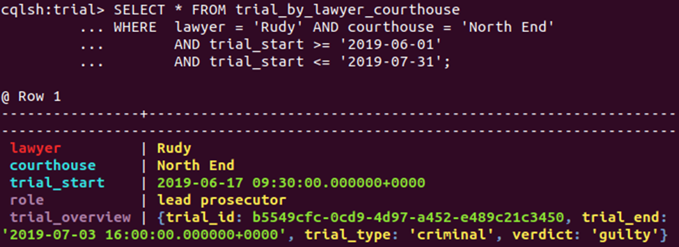
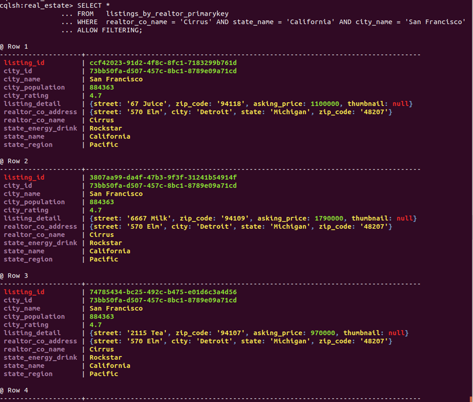
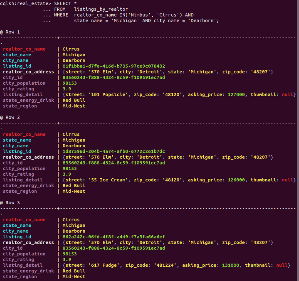
As an example, here is a query readout from the CQL shell over a sample table:

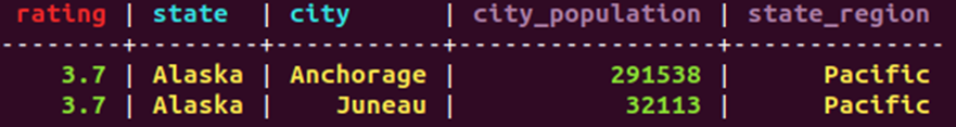
(Partition columns are red, clustering columns are aqua, and regular columns mauve.)

Figure 5 below is the dependency diagram created for the article series problem (and discussed later). The sample table here is bound by three of its functional dependencies, SC → G, S → N, and CS → P where S: state, C: city, G: city rating, N: state region and P: city population. Of them, only data involving FD S → N can be duplicated between rows in the same partition. The design is viable and the two rows shown don’t violate the FD – although they could.

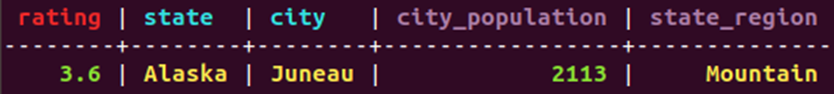
Erroneous input into a different partition as above, however, causes all three FDs in the table to be violated. As you know from the previous article, there is no mechanism in the Cassandra system to prevent this and finding it with CQL only can be difficult.

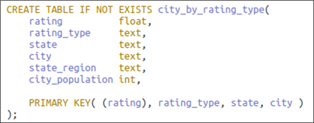
FDs can change as requirements are better understood. Say SC → G becomes ISC → G, where “I” means “rating type;” prepend it to the clustering column list:

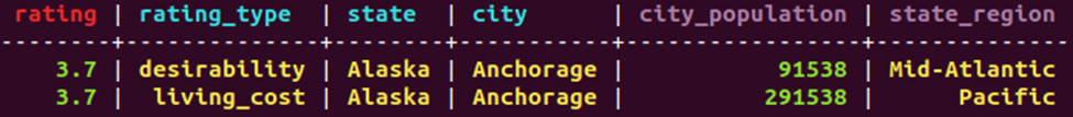
As with SC → G, dependency ISC → G can only be broken in rows spanning partitions, but S → N as before along with CS → P now can break in the same partition:

This sketch applies both to one-to-many and one-to-one relationships – the functional dependencies as they occur in the unified relation. It also applies, in a way, to the many-to-many relationship as well.

Many-to-Many

Not discussed in the series so far is the common case of the many-to-many (m:n) relationship. The restrictions placed on attribute sets for functional dependencies in the primary key – see section Placement of Functional Dependencies in Part II – don’t apply to key attributes on either side. Consider this simplified ERD snippet:

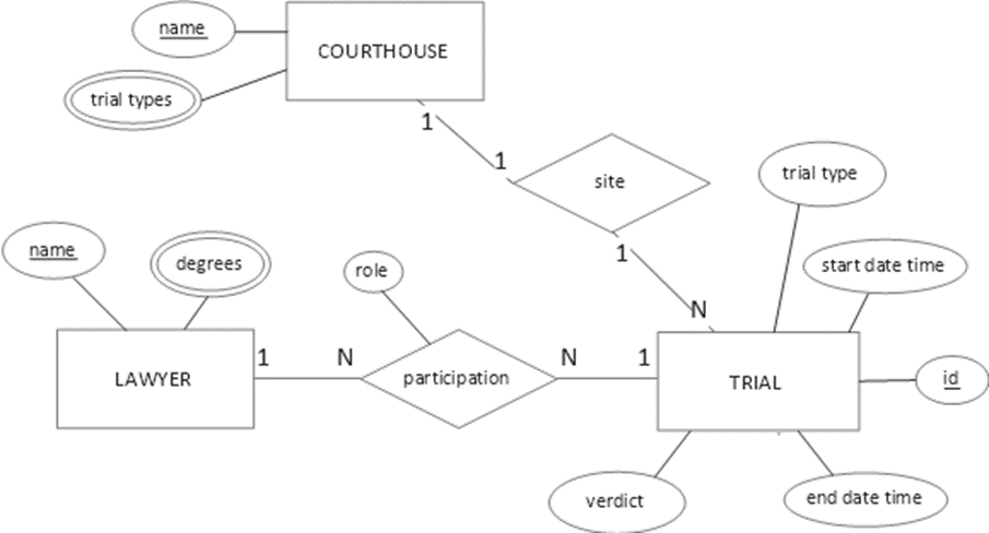
Figure 1. Conceptual trial model (Chen notation)

In the unified relation, the “site” one-to-many relationship establishes an FD with trial ID as determinant and courthouse name as dependent.

In contrast, the “participation” binary m:n relationship does not establish the m-side or n-side attributes as FDs in the unified relation. The relationship indeed combines two one-to-many relationships. However, they are not mutually independent and cannot be modeled in ERD as two distinct relationships. As a result, the lawyer identifier does not functionally determine trial attributes, nor vice-versa.

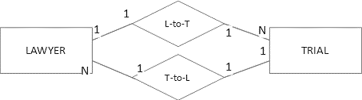
Figure 2. Not equivalent in meaning to Figure 1 “participation” m:n relationship

However, in relational and Cassandra modeling, the two one-to-many relationships are directly applicable. Say “lawyer name” and “trial ID” are both in the Cassandra key. If lawyer Stuart appears K times in combination with different trial IDs in “participation”, then pairings of Stuart and trial ID in the key yield K duplicates for each associated Lawyer entity attribute placed as a regular column. The n:1 relationship with the Trial entity is parallel.

Placing identifiers for both lawyer and trial in any part of the key in either order is always correct. They can both be in the partition, and their dependents made static (if clustering columns exist). If one or both is a clustering attribute(s), the second identifier implies expansion in the conceptual row nesting disc layout (see Part I).

For example, take C to mean courthouse, L lawyer and T trial identifiers. Given they are all in the key, restrictions are that C comes before T because T → C and T and C cannot both be in the partition for the same reason. Functional dependencies and m:n relationships mix easily in the primary key and table. Legal keys, then, include ((C)TL), ((C)LT), ((CL)T) and ((L)CT). Satisfy yourself that every successive clustering attribute in each key expands row nesting.

Any n-ary degree m:n relationship can cause significant redundancy within a table. Say the key is ((S)LCT) where S is the state wherein the courthouse resides (C → S). If lawyer Rudy has appeared in three courthouses and argued in three trials in each, then needed attributes in a relationship with Rudy appear as regular columns in nine rows. Attributes related to each courthouse are duplicated three times. If Rudy has a role in trials in more than one state, this redundancy is spread over multiple partitions.

This section concludes with a final example in logical and physical design based on Figure 1. Here is the access pattern for which to solve:

Q_n. Find trials started in a time frame by courthouse and lawyer

Notice first that courthouse and lawyer are in a m:n relationship.

To satisfy the access pattern’s implied range queries, Trial’s non-key attribute “start date time” – lower case “t” – must be a clustering attribute. It must follow lawyer and courthouse IDs in the key since by CQL rules, once a clustering column is sliced by an inequality operator in the WHERE clause, no clustering columns following it in the list may be restricted.

The trial ID (T) could follow t in the key because T → t. still, it seems that given a lawyer and a point in time, the combination should yield a trial, i.e. the FD Lt → T. This cannot be deduced using Armstrong’s Axioms. It requires a new business rule: A lawyer can start only one trial at a time. Now T must be removed from the key and made a regular column along with its related attributes (precisely because Lt → T).

Logical key possibilities then are ((C)Lt), ((CL)t) / ((LC)t) and ((L)Ct). The first ((C)Lt) would create the largest number of rows on fewest partitions, and the second, ((CL)t), the smallest number on most partitions. These are considerations for the physical stage and somewhat in the logical as well. The decision is made to use key ((L)Ct).

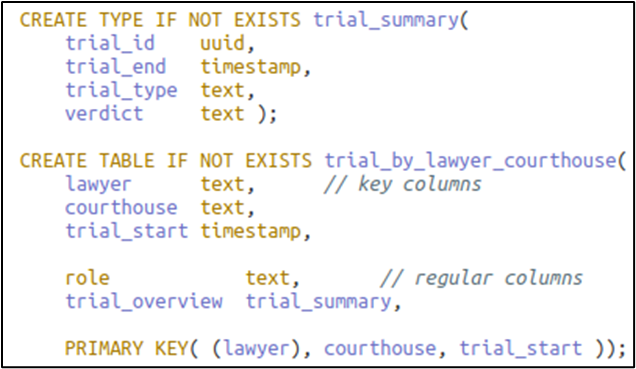
Figure 3. Table for intermediate-sized partition

Access pattern Q_n can now be satisfied with equality or range queries over time:

This table may be part of a two-pass query, the second retrieving documents and other trial details given the trial ID; refer to the application workflow.

Attribute Closure: Implications for Cassandra Design

This section returns to analysis by functional dependencies only.

These next subsections dovetail with techniques for discovering further properties of Cassandra tables and primary key design. The first presents a diagram of functional dependency relationships inferred from the SQL Server normalized physical design in Part I. The second, a code module that references the diagram as input for computing attribute closures given sets of initial attributes.

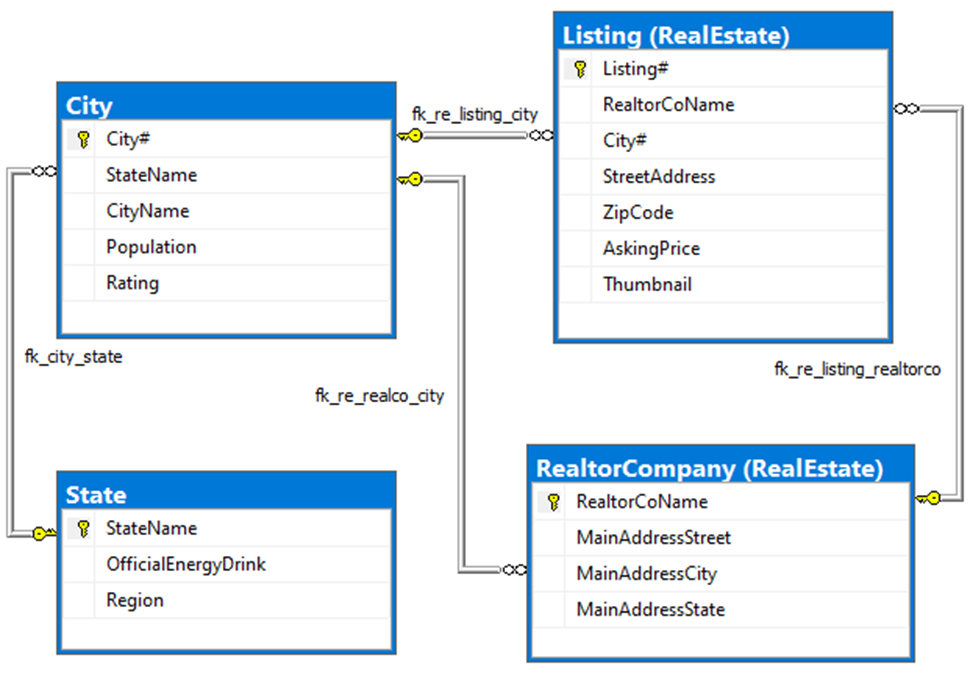
Figure 4. Normalized physical design (Part I)

The Functional Dependency Diagram

Functional dependencies placed into the unified relation come from the primary and alternate keys, the latter not shown by the SQL Server design tool. One FD not included (the dotted arrow) indicates that realtor location additional data is not relevant to the series problem’s access pattern.

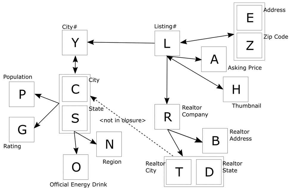
Figure 5. Functional Dependency diagram from normalized schema

I’ve abbreviated attribute names to single letters, intuitive when possible. Herein I’ll often refer to attribute names as their single-letter counterparts.

The arrow recipients in the diagram are the dependents, and the arrows emanate from the determinants. Composite determinants are grouped in boxes; the double arrow implies a (1:1) relationship, I’ve elided redundant arrows in such relationships and so on. Not surprisingly is the double arrow between Y and SC (City# and State/City names}. (In the SQL Server logical design, the latter was key for the City relation, and in the physical design, the surrogate City# was added as primary key, and the composite was enforced as alternate key). Follow the arrows to see the partial and transitive dependencies.

By visual inspection alone, you know that L, EZ and H functionally determine, directly or transitively, all other attributes. As each is irreducible, each is a candidate key. The diagram is an important artifact. What is needed, though, is an additional tool for proving certain properties of key and table design choices.

The Attribute Closure Module

The elementary code module below does a closure over an initial set of attributes in the unified relation given the relation’s set of functional dependencies. Its purpose is to determine which key attribute additions make for “uniqueness,” and which attributes become static or regular attributes in different Cassandra key design choices. This analysis is essential for larger, more complex relations.

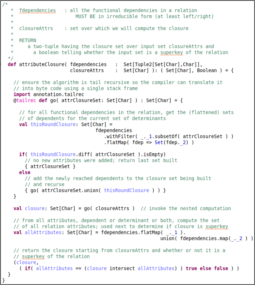
Figure 6. Attribute closure function

I wrote the solution in Scala. If you’ve done C# or C++ or Java or other imperative/object-oriented language, the algorithm shouldn’t be difficult to follow. The one twist is that Scala also fully supports functional programming. This style allows functions to appear wherever a variable could. Thus, I’ve nested the “go” function inside function “attributeClosure” rather than placing it separately as a private function in the wrapper class (or object) where it most certainly wouldn’t be reused by other methods.

Essentially, each recursive invocation of the inner function uses set operations to glean the next set of dependent attributes implied by two structures. The first structure is the invariant set of FDs (“fdependencies”) as passed into the outer function. Second, the inner function’s parameter (“attrClosureSet”): the set of already captured attributes, acting as the source of possible determinant combinations. This set is initialized from parameter “closureAttrs”.

At each recursive step, if new (dependent) attributes are added to the closure, iteration continues. If not, the inner function returns the closure to the outer. The outer then returns a two-tuple consisting of the closure plus the Boolean decision as to whether the initial attribute set attrClosure is a superkey for the relation.

The dependencies input, “fdependencies”, mirrors the dependency diagram (Figure 5):

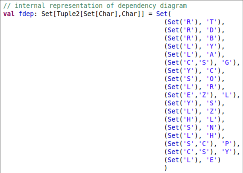
Figure 7. Sample structuring of functional dependencies in Scala

The input dependencies for this implementation are irreducible, meaning it meets these criteria: a) right-irreducible: each dependent is a singleton; b) left-irreducible: each determinant set is minimal; and c) there are no trivial FDs (A → subset(A)) or FDs derivable from other FDs. In this implementation, c) is waivable. For any implantation, b) is required.

Beyond the design stage, functional diagrams and this algorithm can be instrumental in tracking down FD data errors in tables, e.g. via a Spark application.

Sample run readouts are deferred for the next section.

Solution Space

The series began with the stated goal of transforming a normalized SQL Server schema (Figure 4) into a Cassandra table designed for this access pattern:

Q_k Find listings for a realtor company in a city

Realtors and cities are in a m:n relationship, so their ordering in the key doesn’t matter.

The solutions can reference the results of applying the FD set in Figure 5 and initial attribute sets to the closure function in Figure 4.

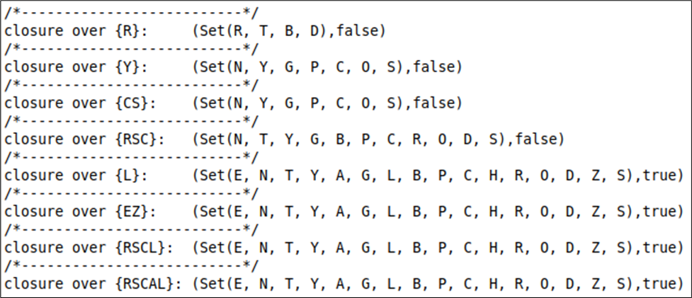
Figure 8a. Sample closure runs (eclipse software)

Incidentally, Scala runs in PowerShell; see readme.txt file included in the downloads for instructions on installing and using Scala.

Figure 8b. Sample closure runs

I’ll repeat a central point. The closure is an important method for deciding whether and which attributes need be appended to the primary key for “uniqueness”: i.e. to cover all attributes using minimal collections. This is not the same as making the key unique; the Cassandra key is always unique. Collection types make this possible. If the key were R, e.g., its singleton row would have collections structured over combinations of CS-Y and L and their related attributes. You saw this in Part II.

To satisfy the access pattern, RSC or RY – not both! – must be in the key as search attributes. There are now two decisions to make. The first, as you expect: is it RSC or RY? In consultation with the analytics team, secondary stakeholders to this OLTP database, they would prefer RSC as it simplifies querying over RS by itself.

The second concerns selecting partition attributes. In the logical model, R by itself is sufficient; in the physical, assume the row count and size are manageable and performant, so the base key remains ((R)SC). Closure results indicate, among other conclusions, that attributes T, B and D must be static.

This discussion ends what has been considerable background, except for one more tool.

Design A: The Minimal Superkey

As per the closure, L is a relational candidate key. Could it be the partition and full primary key (no clustering attributes) for its singleton row while satisfying the access pattern?

Figure 9. Possible logical model from the KDM

The Kashlev Data Modeler (KDM) is a tool for automating Apache Cassandra logical and physical designs (see references). It produced the logical design above given key L and an ERD. KDM uses Chebotko symbols to identify Cassandra column types. The “K” is for partition column.

Here is the actual table definition in CQL I devised (not from KDM):

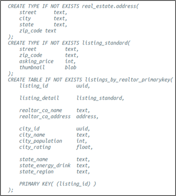
Figure 10. Physical design featuring minimal superkey and UDTs

This is the query showing the first three rows returned (almost):

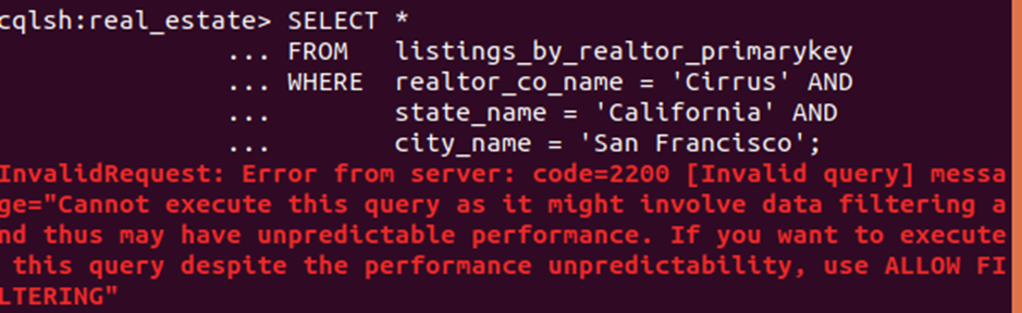
Well, the CQL shell tried. The error message with terms “data filtering” and “unpredictable performance” means this: The system can’t initially use the WHERE clause predicate conditions but must visit every singleton row in every partition – essentially, a table scan. Only then can It filter out rows not meeting the (RSC) search conditions. Depending on several factors, the query may involve many or most or even all cluster nodes, potentially vitiating the excellent performance of which Cassandra is capable. Then again, performance may be fine – just a warning and you can append the ALLOW FILTERING clause. Still, it’s an unacceptable warning for the main access pattern for which a table was designed.

Secondary indexes help in some cases but not this one. In short, the table is too highly transactional, and the ALLOW FILTERING clause would still be required. I placed indexes on all RSC columns and Cassandra did use the one with the highest selectivity – the one on the city name:

Among several examples of data duplication here is owing to dependency CS → GP (city to rating and population), or alternatively Y → GP (city UUID to same). Thus (San Francisco. California) yields (4.7, 884,363) for every listing row in this city in different partitions. This particular redundancy is better managed in the remaining solutions, which build from the base ((R)SC).

I stress again that the major problem is the table scan. Regardless, you may have concluded that the candidate key approach given Q_k would work better later in the application workflow with a different access pattern. There, its attributes can be more specific to the listing such as a video, floorplan, and information about schools.

Design B: Key Sans Uniqueness

In this solution, the key is ((R)SC). The redundancy owing to CS → GP is eliminated. However, as per closure results (Figure 8), it can’t reach all attributes – specifically, those for the listing. Since the listing identifier functionally determines RSC, the solution requires placing the listing identifier and its directly reachable attributes coalesced into a collection:

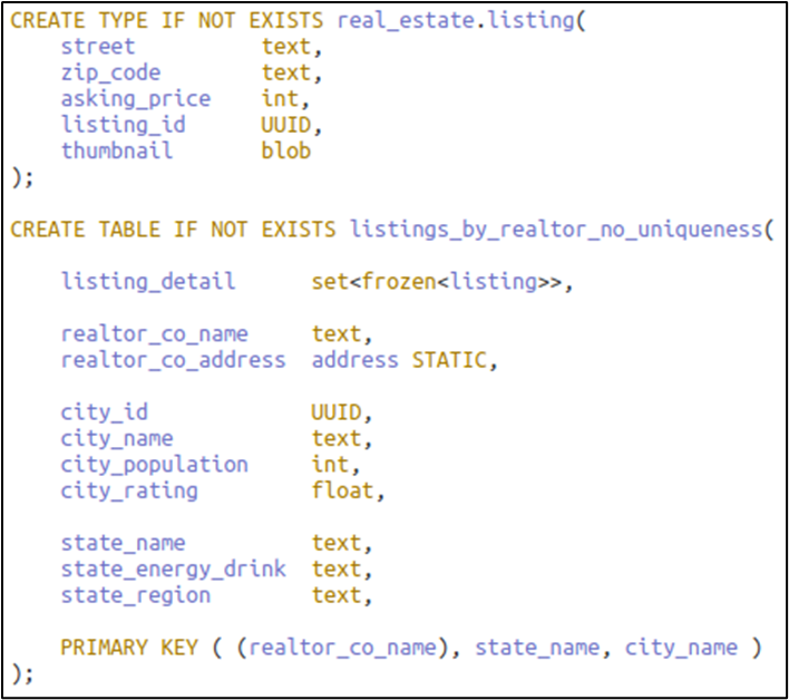
Figure 11. Physical design where key lacks uniqueness column

Read this to mean that a realtor company in a city has zero or more listings.

Notice that given R → BDT and ((R)SC), Design B introduces static (UDT) column “address” (Figure 10). The static designation ensures that address is not repeated into each row in a partition. It further enforces the first rule of functional dependencies as introduced in Part II: a determinant (R) and its dependents (BDT) can never appear together in the partition key.

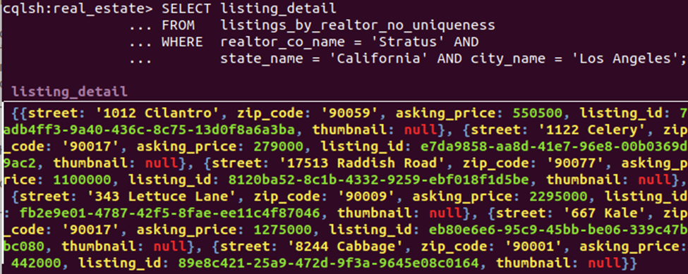
The query result shows listings for a single row. For the testbed, the design collapses six individual listings into one row. A realistic example could have hundreds of listings. In querying, the client potentially can access numerous rows. The size of the return set (each row listing collection being indivisible), the highly transactional nature of the collection and other factors render this solution unsuitable.

The recommendation is to use collections when data is smaller, bounded and need little updating. Think, as a simple example, book authors in a list.

Design C: The Non-Minimal Superkey

More to standard is appending the listing identifier as uniqueness attribute to make ((R)SCL); logical and physical designs are as follows:

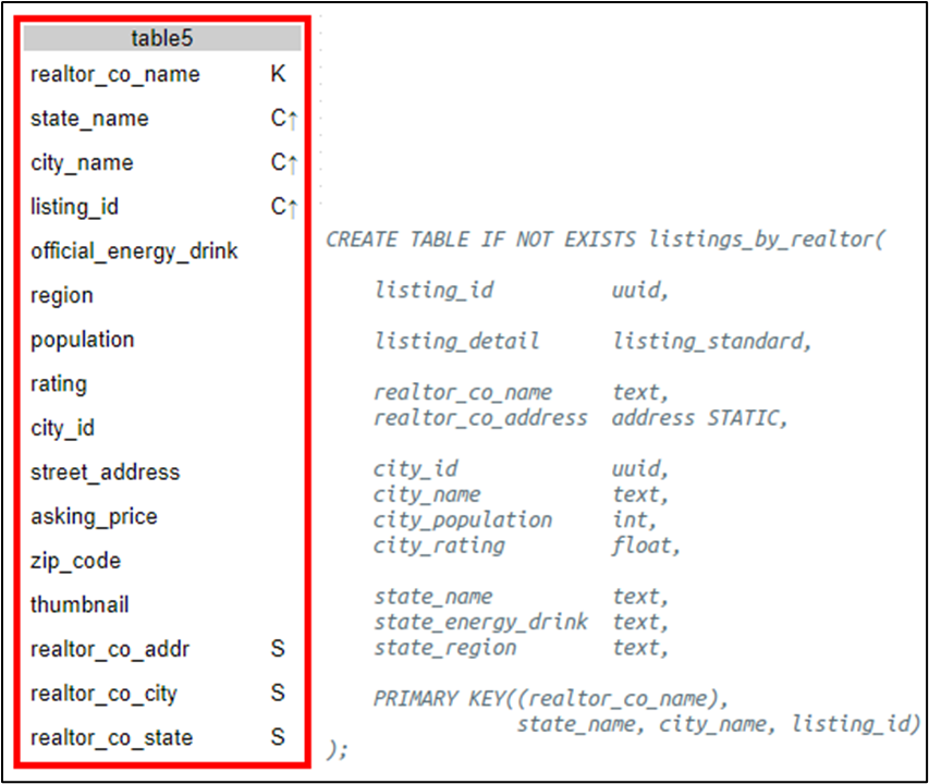
Figure 12. Recommended designs for access pattern Q_k

Continuing Chebotko logical notation, the C↑ is clustering column ascending order, and the S is static.

By constraining on the prefix of key columns short of listing ID, the query satisfies Q_k as the first three rows returned from the sample query show:

Listings that were compressed in Design B are now each in their own row. No less information is retrieved – in fact, the design accounts for more redundancy as seen in regular columns for state and city. Unlike B, however, row modifications in this highly transactional table are simpler and safer, and clients can take advantage of paging of listings over realtor-city pairings.

Design D: The Non-Minimal Superkey with Additional Ordering

Sometimes a table is correctly designed but still falls short of needs. The problem, then, is the access pattern itself: it needs a fuller description.

Perhaps searching on or organizing data by zip codes, or range querying over asking price is also desired. Say the access pattern is altered thus:

Q_k Find listings for a realtor company in a city sorted from least to highest asking price

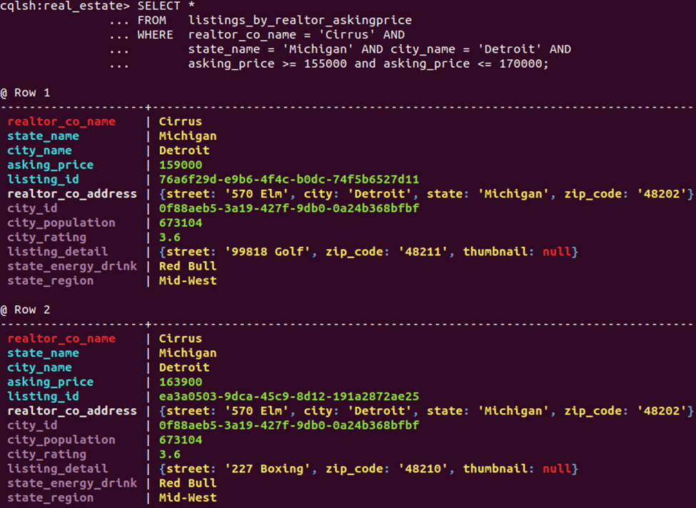
Starting from Design C, pull the asking price out of the listing standard UDT (Figure 10) and wedge it between the search and uniqueness columns: ((R)SCAL):

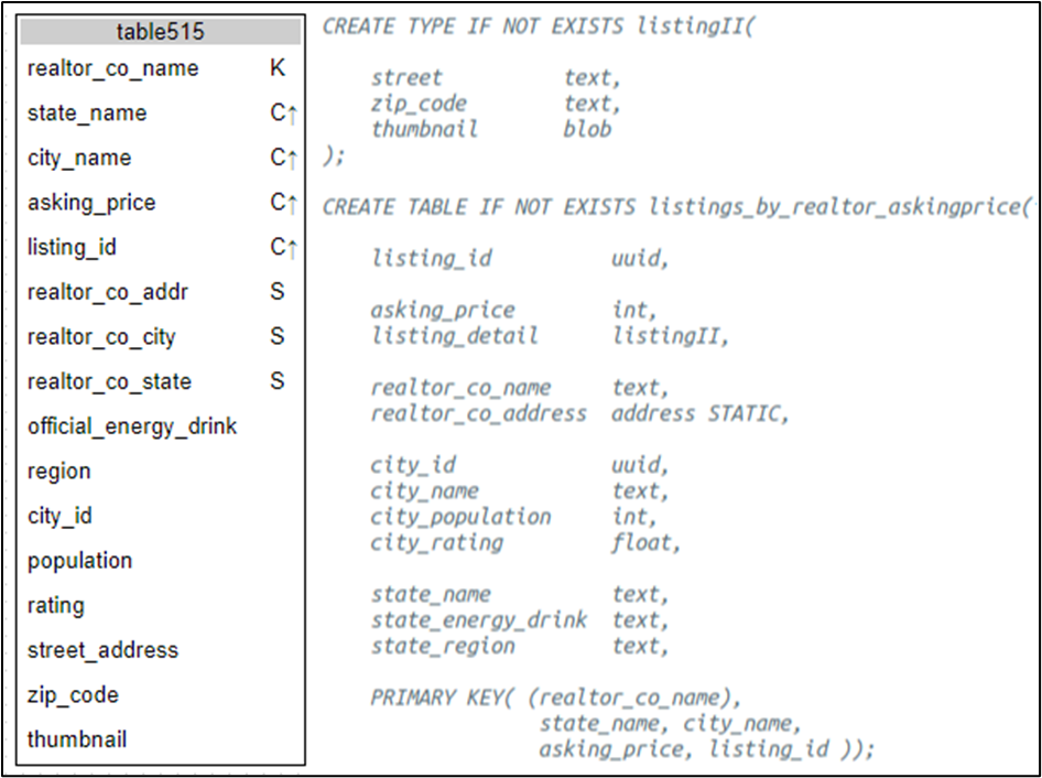
Figure 13. Logical and physical designs with ordering on asking price

Client software can now page through the table already sorted by price, or do a range query as seen here:

Always think conceptual row nesting on disc. As a general rule, inserting a new attribute(s) into the clustering list must expand row possibilities for key attributes defined before it. You may want to review Part I for specific rules on clustering column type and placement.

Last Word

Relational SQL Server and NoSQL Cassandra are meant for different use cases. As such, there may be more differences than similarities between them. You’ve seen a number of differences, including rules for key design and the ability to enforce integrity constraints. I won’t list them or introduce others here, but I will leave you with one final thought.

If conventional wisdom says that the relational model and theory has no valuable insights for NoSQL systems, do you (still) believe it?

References

J. King, “DS220: Data Modeling,” https://academy.datastax.com/resources/ds220-data-modeling, a DataStax Academy online video series course on Apache Cassandra.

DataStax Documentation, “CQL for DataStax Enterprise 6.7,” https://docs.datastax.com/en/dse/6.7/cql/cql/cql_using/queriesTOC.html, primary key and querying.

J. Carpenter, E. Hewitt, Cassandra The Definitive Guide Distributed Data at We Scale, 2nd ed. Sebastopol: O’Reilly Media Inc., 2016.

A. Kashlev, “The Kashlev Data Modeler,” http://kdm.dataview.org/, an online automated tool for developing Apache Cassandra logical and physical designs.

DataStax, “Data Modeling in Apache Cassandra 5 Steps to an Awesome Data Model,” https://www.datastax.com/sites/default/files/content/whitepaper/files/2019-10/CM2019236%20-%20Data%20Modeling%20in%20Apache%20Cassandra%20%E2%84%A2%20White%20Paper-4.pdf?mkt_tok=eyJpIjoiWmpnMk4yWTVaR0l6WTJOaiIsInQiOiJWTFQyYW5LRkljSWt2Q28xSDR5RXBBNmNlM1pLbThFTFFwSHJLd0E1NXdYM2VmbHJaam1HelFSSThCYW1JRVZVSE9uM1YzTmYzbDVTUlB5c3RESlNyTTJYMSs3bE90QlNiVmRrZkg2ZDZINlYrS1MralJ1Zzh2K1pKNVZ0K0g2aSJ9, White paper .pdf.

C.J. Date, An Introduction to Database Systems, 8th ed. Boston: Pearson Education Inc., 2004, esp. Chapter 11 Functional Dependencies.

D.R. Howe, Data Analysis for Database Design, 3rd ed. Oxford: Butterworth-Heinemann, 2001, esp. Chapters 9 Properties of relationships and 10 Decomposition of many:many relationships.