Interpolation is a mathematical technique which was popular before we had a lot of cheap computing power. The basic idea is that if you’re given a set of data and looking for a value in the same range, you can interpolate it to get a reasonable estimation for the value that is not actually in the set.

If you can find an old calculus, finance, statistics or algebra book, they had lookup tables in the back. Remember that the only computational tools students had back then were pencil and paper or a slide ruler. If you wanted to use a pencil and paper, you had to know what formula to use. If you use the slide ruler, you can only have three decimal places in your answer (yes, there were a couple of over-sized specialized slide rulers which could go as high as four or five decimal places. They were very expensive). But if your slide ruler didn’t have a particular function you were trying to compute, it was hard to get even the three decimal places.

When you try to approximate a value outside the range of your set, that’s called extrapolation. It’s a different topic and requires a slight leap of faith.

Nearest-neighbor interpolation

The nearest neighbor algorithm Is the simplest form of interpolation. It creates a value which is nearest (or equal) to a known value in the table. It does not consider the values of neighboring points at all, yielding a piecewise constant interpolant. This sounds fancy, but it really isn’t. Consider a lookup table for the size of a box for packing an order from a customer, based on the weight or count of the contents. If the items you’re selling are pretty much the same volume per unit of weight in the same shapes, then this might be just fine for your work.

For example, if I own a video store, my packages stand a very good chance of using a limited set of sizes corresponding to the number of DVDs in a shipment. This is because DVDs tend to be close to the same shape and size. The algorithm is straightforward to implement; divide the total number of DVDs in the shipment, pick the smallest boxes that will hold that number of DVDs. For example, if somebody orders 15 discs of “Law & Order”, you can pack it in one 10-unit box and one 5-unit box. This is based on the assumption that these two packages are cheaper than three 5-unit packages which may or may not be true in the real world. Or maybe a 20–unit package with a lot of Styrofoam in it could be the winner. Even worse, it might be possible that sending out 15 single–unit packages is cheaper! Many decades ago, I ran into such a situation when a promotional item was my choice for Christmas gifts. The premium item being offered was already packaged in mailers, so the cost of repacking them would’ve been complicated and prohibitive.

But if I am a general merchandise store, I’m not going to get a fishing pole into the same box that I used for a pair of shoes of the same weight. I ran into a problem like this decades ago, with a picklist for a mail-order barbecue company. Essentially, each order generated a pick list of the various items which were sent to the shipping department be put in boxes with the appropriate dry ice and insulation. The shipping department had to pick the proper size box to use along with the amount of dry ice needed. A bad guess could mean that an order had to be unpacked, put in a new box, and reprocessed. Since much of their Christmas rush was done by temporary help, who lacked the experience to make a good guess, this was getting to be very costly. The first approach their consultant had taken was essentially to play three dimensional Tetris with the items. Ugh!

We found a better approach was to go back to historical data and figure out how many unique orders had been placed in the last several years. As it turned out, we only had 5000 unique configurations on the pick lists. Then within each of the configurations, we picked the smallest box that had been used for shipment and built a lookup table. This became a simple matter of an exact relational division, and a special case (“pack this order by hand”) when the relational division failed.

This challenge is called “bin packing” and “knapsack problems” which is a popular topic in computer science. Generally speaking, there is no guaranteed optimal result.

Linear interpolation

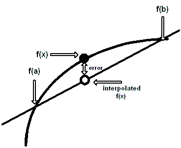
This technique is a way of guessing the results of a function that lies between two known values. Let’s call the two known functional values, a and b, and their results from the function, f(a) and f(b) and try to find f(x), where (a <= x <= b), but x is not in the table. We have to make many assumptions about the function. It has to be continuous over the interval [a, b] and behave smoothly. Thank goodness, most other common functions do behave nicely. It is based on the idea that a straight line is drawn between two function values f(a) and f(b) will approximate the function well enough that you can take a proportional increment of x relative to (a, b) and get a usable answer for f(x).

For example, Let’s assume we have a table of census figures for the years 1970, 1980, 1990 and 2000, and we want to estimate the population for the years 1975, 1985 and 1995. Assume that population growth between the years we know was linear and hope that there were no spikes in births or plagues in between. This method was used by Babylonian astronomers and by the Greek astronomer and mathematician, Hipparchus (2nd century BCE). The algebra looks like this:

This can be translated into SQL as simple algebra.

The CASE expression in the divisor is to avoid division by zero errors when f(x) is actually in the table, and we are only looking at one point.

Nonlinear interpolation

Linear interpolation assumes a well-behaved function, which grows in a linear fashion. It is quite possible that something may have rapidly increasing growth. Consider a table of a population census for the years 1960, 1970, 1980 and 1990. This model assumes the population for the year 1975 should be halfway between 1970 and 1980. But the truth might be that there was a period of really rapid population growth in the late 1970s because of massive immigration, an increase in birth rate, or other factors. Likewise, we could have massive population decay due to a plague, famine, war, or other events. You can actually see this pattern in the parish records of England. With the rise of capitalism, a population that had been in a “sawtooth pattern” for centuries suddenly changed to uninterrupted growth. It wasn’t that people began to breed like rabbits, but they stopped dying like flies.

Common forms of nonlinear data are growth and decay. Simple linear interpolation assumes that the steps within [a, b] are uniform. But growth would assume that as we seek a missing value closer to b, the value of f(x) Increases more rapidly. Now we’re dealing with first derivatives and a little bit a calculus. Those old books I’ve mentioned with the lookup tables also included a value called the first Delta and the second Delta. It was usually a simple formula that added a “fudge factor” to the simple linear interpolation.

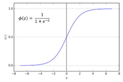
Another common form of nonlinear data is the sigmoid, “S-shape” or Logistics function. If you’ve ever followed a fad, you have seen this sort of data; it starts slow, gains momentum, grows to an inflection or saturation point and then gradually flattens out over time. Consider the sales of incandescent light bulbs, which were replaced by mercury vapor bulbs (“corkscrew lights”) and currently by LED light bulbs. The trick with such growth and decay patterns is predicting where the inflection point is and how long It will take the new technology to replace the prior technology. Failure to do this can leave you with a lot of eight-track cassettes, bell-bottom pants and an unreturnable inventory.

Another form of interpolation is to use polynomials to approximate functions whose computations would otherwise be too complicated. These polynomial approximations are only good over a certain range, and the function for the error is also known. To give an example, log10(x) can be approximated over the range 1/√10 to √10 by the polynomial:

There are several kinds of polynomials that can be used this way. One of the most common is the Chebyshev (also transliterated as Tchebychev) polynomials.

Conclusion

In fairness, given that modern software has pretty good libraries for functions, you’re probably not going to do a lot of floating point arithmetic from scratch. In fact, given that most of you will be doing commercial rather than scientific work, you probably will do most of your computations with decimal data types and will follow legal requirements that governments, auditors and accountants (EU requirements and GAAP rules) have set up for you. But I still feel, however, it’s good to know such things exist, in case you ever have to go to a reference book and figure out what’s going on. Even if a professional doesn’t use them very often, a professional ought to know what they are and where to find them.

References

Cody, W. J. (1970). “A Su.rvey of Practical Rational and Polynomial Approximation of Functions”. siam Review. 12 (3): 400–423. doi:10.1137/1012082

Hart, John F. (1978). “Computer Approximations:SIAM series in applied mathematics”.ISBN 0–8827–642–7

Martello, Silvano and Toth Paolo.  “Knapsack Problems: Algorithms and Computer Implementations” by (ISBN 0–471–92420–2). The book is old, a bit heavy on math, and the computer code given the back is in FORTRAN. But the text uses an Algol family pseudo-code that should be fairly easy for anyone to read and turn into a modern procedural language. You can download it at http://www.math.nsc.ru/LBRT/k5/knapsack_problems.pdf.

RAND Corporation.  “Approximations for Digital Computers”  (1955).  This has been reprinted as a classic ISBN 978-0691653105. You might remember the RAND Corporation as the people that gave you a table of a million random digits (also still in print).