
Part I: Problem Space, SQL Server Simulation and Analysis
This article covers an interesting approach to a software problem. The software to be built must transform data in an operating system file. Would it make sense to include SQL Server in the development environment?
Solving problems first in T-SQL provides result sets against which software results can be compared. Adding to that, query execution plans may serve as blueprints for software development.
In this Part I of the series, I’ll fashion business rules, requirements, and sample data into a denormalized table and query. The query’s WHERE clause includes several logical operators, but its query plan is trivial. To get one that can serve as a software design model, I’ll rewrite the query’s logical connectives as their set operator equivalents. The new query plan is more complex but suggests a logical approach for the software effort.
In Part II, you’ll see T-SQL components realized as structures you know: lists, sets, and maps. What you may not know, though, is how to code algorithms declaratively – e.g. without long-winded loops. The software makes extensive use of map functions, which take functions as arguments and are supported to varying degrees in many Visual Studio languages.
For this article, you’ll need development experience in a relational database and some knowledge of relational theory. For the next, any experience in an imperative or declarative language suffices. Though I’ve written the code in Scala and solely in the functional paradigm, I hope to present just enough background for you to grasp the core strategy of the solutions.
You can download the complete files for both articles.
Problem Space: Ice Cream
Ice cream manufacturers and retailers, whom I’ll refer to as makers, purvey many flavors. Here are the business rules:
- There is a many-to-many relationship between makers and flavors.
- There is a many-to-one relationship from flavor to base flavor (functional dependency: flavor → base flavor).
The term base flavor is an article device not an industry standard.
Participation is mandatory in both. This illustration shows the relationships for five of twelve rows from the operating system file in entity-occurrence style:
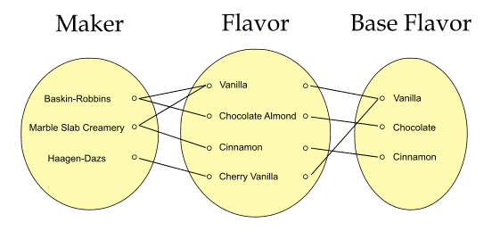
Figure 1. Many-to-many and many-to-one relationships
This is the statement of the data manipulation requirement to be done on the operating system file in software:
For rows in which maker names end in ‘Creamery’ or the base flavor is Vanilla, further restrict these to their flavors being Mint, Coffee, or Vanilla. Return result for all three columns.
The reference to maker name of suffix ‘Creamery’ will result in a non-searchable argument (SARG) that will be handled transparently by the T-SQL but must be addressed directly in the software.
There is a subtle incongruity between the business rules and the data transformation requirement. Do you see it? The file and table will have the same twelve mockup rows but imagine thousands in a real project and how this could impact performance. I’ll point out the issue and resolve it later in a query and take what was learned when developing the software.
Problem Space: The Ice Cream Database
The goal of the table in the simulation database simply is to mirror the data in the file. The many-to-many relationship implies that (Maker, Flavor) is the sole candidate key. Since flavor → base flavor, the table would not be normalized; in fact, it is an intersection table in violation of 2NF. Further, there are no foreign keys or other tables as they would add nothing for the software design.
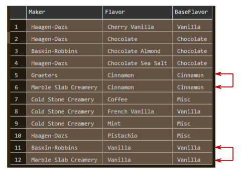
Figure 2. File sample rows having redundancies – not in 2NF
Denormalization is visible in rows 5 and 6 and in 11 and 12. The non-clustered covering index (added post-population) will give a better query execution plan (query plan). More importantly, it will be matched by a key structure in the software – I’m tuning the database only to the extent that it will be relevant later.
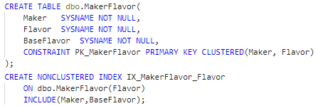
Figure 3. Denormalized intersection table and covering index creation
All database work was done in Azure Data Studio connecting to a local copy of SQL Server 2019. The script is in the download.
Solution Space: T-SQL Queries
The first goal is to create a result set against which the software result can be verified. Adhering to the business rules and requirements, the query constrains on four logical (Boolean-valued) operators, LIKE, IN, AND, and OR:
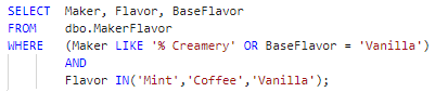
Figure 4. Original query that creates rowset for software verification
This is the query outcome over the sample rows:
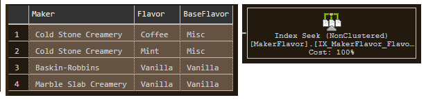
Figure 5. Verification rowset with single-step query plan.
The Index Seek operator over the covering index expands the IN() operator, which implies logical OR, into Seek Keys (for a range scan count of 3), and further constrains on the Predicate as expected:
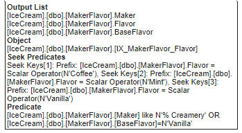
Figure 6. Bottom part of expansion for Index Seek operator
All is correct to this point, and I can convert the index into a structure that will be used twice in software. However, the trivial query plan is not as useful as it could be. Relational theory is based on set theory, and the query rewrites next will more directly reflect this. This is important because the transformation algorithms in the software will all be set-based.
Query Rewrite I
The second goal, as you recall, is to fashion a query whose query plan will serve as a model for the software design. The trick I’ll employ is to replace the logical connectives OR and AND with their T-SQL equivalent set operators UNION and INTERSECT.
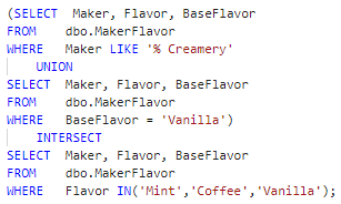
Figure 7. Query rewrite using set-based operators
It produces the detailed query plan I’m looking for:
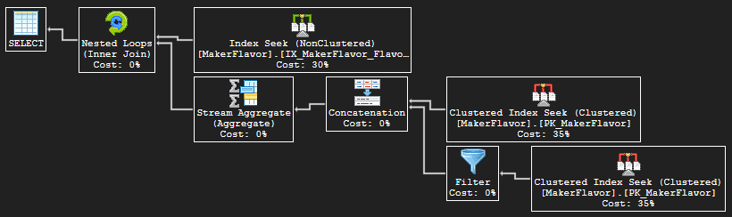
Figure 8. Query plan for Figure 7
The outer input uses the same non-clustered covering index and Seek Keys for range scans (scan count remains 3) as the original query but without the Predicate. Instead, each outer row directly joins via Nested Loops (Inner Join) on all columns to the rowset produced by the union of the Creamery and base flavor rows (discussed next). The Nested Loops operator, then, accomplishes a row-by-row set intersection.
In the inner input to Nested Loops, the upper Clustered Index Seek on the primary key is for the LIKE(% Creamery) condition. Although the value to the LIKE logical operator is a non-SARG, a true index seek range scan (not table scan) is done on each outer row’s (Maker, Flavor) prefix, during which the LIKE Predicate can be applied. The lower Clustered Index Seek parallels the upper, differing only in the predicate condition: BaseFlavor = N‘Vanilla.’ Since the Inner Join is done on the superkey – i.e. all columns – and since flavor → base flavor, either lower input branch can produce at most one row. If both produce a row, they must, therefore, be the same row.
The Concatenation simply appends one output to the other – think UNION ALL in T-SQL. To get the T-SQL UNION, then, the Stream Aggregate (Aggregate) operator collapses duplicates via grouping (and no aggregate expressions are computed). Specifically, both Concatenation and Stream Aggregate show only the same Output List, which consists of column header Union 1004, Union 1005, and Union 1006, and their rows are returned to the query.
This query plan lends all the information needed to create index simulators and filter and map operations and algorithms in the software. An optimization, though, remains unaddressed – so almost all.
Query Rewrite II
There is no index on the BaseFlavor column, but in the middle subquery from Figure 7 above, BaseFlavor is constrained on value ‘Vanilla.’ This suggests that the lower-level software might need a data structure(s) and algorithm(s) to support the restriction. To start the analysis, I’ll create this covering index, which parallels that on the Flavor column:
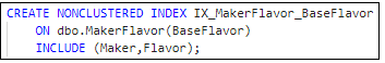
Figure 9. Covering index on BaseFlavor key
The proposed index has no effect on the query plan in Figure 8 above, nor the original query plan in Figure 5. This is not proof, though, that separate resources are not needed in software to enforce the restriction.
The next illustration shows the subquery run in isolation. A minor point is that the Query Optimizer chooses an Index Seek on the new index in place of an Index Scan using IX_MakerFlavor_Flavor. The central point is that subqueries that form part of a larger, single-statement T-SQL query will be translated into individual software resources that can and will be accessed in isolation.
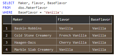
Figure 10. Query in lower half of UNION run in isolation
Now rerun the query but this time constrain the ‘Vanilla’ value by the Flavor column:
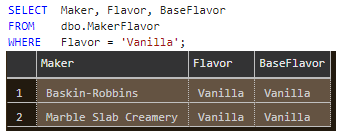
Figure 11. Constraining on Flavor column yields two fewer rows
This is not an idle thought experiment. The former result set contains two extraneous rows – column Flavor values being ‘French Vanilla’ and ‘Cherry Vanilla’ – that are not in the result set from Figure 4. The software effort needs a decision as to which constraint to enforce. Whether in queries or software transformations, performance is better served when rows not needed are culled early. The question I posed early on regarding the mismatch between the business rules and requirement can now be restated: Can the restriction on BaseFlavor be replaced by that on Flavor and still be correct?
Constraining on the one side of a many-to-one relationship as does the top query form (BaseFlavor) is not wrong per se but is the root of the performance issue here. A business rule, however, signals the solution. The second states flavor → base flavor. Given this, and since the query’s set intersection operation removes rows not matching on the Flavor column, the T-SQL can constrain on the many side (Flavor) without affecting correctness. The implication for software is that it obviates the need for special structures – those for simulating the proposed index to start the section – and handling (algorithms), as will be made clear in Part II.
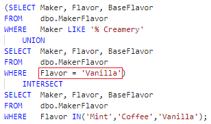
Figure 12. Query in final form
Testing: A Note on the Sample Data
Say set A denotes the rows produced by the query that restricts on the three flavor names and set B the rows from the union of the two other queries. Given the sample data, it happens that A B and hence B ∩ A = A. Therefore, the query on flavor names alone yields the same result as the full query and the knowledge of which can aid testing.
It is important to realize that this outcome is entirely data-dependent. The proper subset relationship may not hold over an operating system file having different data, and the software will make no assumptions regarding this limited analysis. In general, it is never a good idea to deduce business rules from data that can change over time. With that caveat in mind, sample runs done here and in software over these rows can only boost confidence in results.
In Conclusion
You saw how business rules and software requirement were mapped to a single intersection relational table in which normalization and referential integrity were nonessential. The initial query on the table provided the rowset against which the software result could be verified, but its query plan was inadequate as a pattern from which the software design could proceed.
Rewrites using T-SQL set operators did yield a query plan as software blueprint and provided other insights as well, chief among them the optimization of the base flavor column.
Last Word
Neither loops nor branches were used in any of the T-SQL work, but that doesn’t mean they aren’t there. They are – visible underneath in the query plans, which describe the process steps (operators and data flow) the SQL Server database engine follows to produce results. A salient example of looping is the Nested Loops operator used in the T-SQL rewrite query plan to match each outer row to an inner row, i.e. perform the INTERSECT. This style of coding, in which the logic of the computation is expressed rather than the lower-level control flow detail, is declarative programming, and is a major theme of this series. (The latter being imperative programming.)
The next article, which uses functional programming to solve the series’ problem, continues in this vein. The logic written to the map and filter functions encapsulated in the data structures is again compact and elegant, even as the compiler translates it to control flow statements.
Translating insights gained here into functional programming will be straightforward but not paint-by-numbers simple. You may have found this discussion challenging – I hope stimulating – and may find Part II the same as well.
This document contains proprietary information and is protected by copyright law.
Copyright © 2026 Red Gate Software Limited. All rights reserved
Load comments