
This is the third article in a four-part series on SQL Server Reporting Services 2012 (SSRS). Part 1, Building Basic Reports, provided a step-by-step guide to basic report creation and Part 2, Customizing SSRS Reports, took a tour of some of the core SSRS features and functions that you’ll need to develop dynamic reports. In this article, you will learn about the rich set of visual features included with SSRS.
Starting with SSRS 2005, Microsoft has included a scaled-down version of the Dundas Chart Control. Starting with 2008 R2, SSRS has an impressive set of visual controls including gauges, indicators, sparklines, and maps. For many people, these features alone offer a compelling reason to adopt SSRS and upgrade to at least 2008 R2.
Getting Started
In order to work through the examples, you will need to have installed and configured SQL Server 2012, SQL Server 2012 Reporting Services, and SQL Server Data Tools (SSDT). The examples will also work with the 2008 R2 version of Reporting Services, in which case you will need Business Intelligence Development Studio (BIDS) instead of SSDT for report development. For further details, please refer back to the Installing and Configuring Reporting Services section of the previously-referenced Building Basic Reports article. The examples will also work with SQL Server 2014, since there were no significant changes in report development with this release.
The code bundle for this article (see the Code Download link in the speech bubble to the right of the article title) contains all the files you need to get started. You’ll need to create the ReportDemo database, by running the ReportingDemoDatabaseScript.sql script.
This article assumes that you understand the basics of creating reports, data sources, datasets, parameters, and grouping. If not, please review parts 1 and 2 of this series before proceeding.
Basic Charts
SSRS is great for displaying data in a tabular or matrix format. You can add hierarchical grouping levels and totals. However, sometimes a picture is worth a thousand words, and as a report developer you will often be asked to display the data in an easily-digestible, visual format. The most basic way to display data, for example ‘sales by year’ or ‘sales by territory’ is with a chart.
Creating a basic chart
Launch SSDT, or BIDS if you are running an earlier version of SSRS, and create a new report server project called ChartProject. Add a shared data source, ReportDb.rds, which points to the ReportingDemo database to the project.
The goal is to design a report that will display the total value of customer purchases on a given date. Add a new report called MyChart.rdl to the project (right click Reports, select Add | New item). Highlight the chart report and then from the left-hand Report Data menu, add a data source called ReportDb that references the ReportDb shared data source. Set up an embedded dataset for the report based on ReportDb and using the following query, which fetches various bits of information pertaining to customer purchases, including the field we wish to “measure”, i.e.PurchaseAmount, over time (PurchaseDate).
|
1 2 3 4 5 6 7 8 |
SELECT Purchase.PurchaseID , Purchase.CustomerID , Purchase.PurchaseDate , Purchase.PurchaseType , Purchase.PurchaseAmount , Customer.FirstName + ' ' + Customer.LastName AS CustomerName FROM Purchase INNER JOIN Customer ON Purchase.CustomerID = Customer.CustomerID |
Listing 1
On your new report, expand out the design area so that you have room to work, and then drag onto the design area a chart control. When prompted to select a chart type, select the basic column chart, as shown in Figure 1, and click OK.
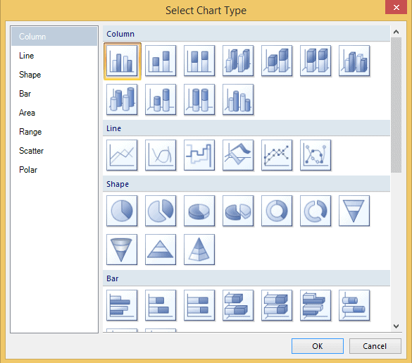
Figure 1
As you can see there are many available chart types, including some 3D charts. In my experience, 3D rendering can distort the heights of the columns, so use caution. Simpler is usually better.
Having selected the chart type, the Chart Data window pops open, as shown in Figure 2. This is where you will add the fields to be measured.
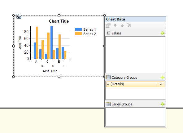
Figure 2
The â Values section is where you add the summary value for the chart, such as “total sales”. On a bar chart like this one, the field you add here will control the height of the bars. SSRS will calculate an aggregate value for the field added to this section, such as a sum (the default), or a count.
Along the horizontal axis, several bars will be displayed. The Category Groups section controls the data represented by each of the bars. Generally, it is a limited set of data, such as several years, the months of one year, territories, or departments. In additions, the Category Group Properties allow you to, for example, add filters or change the sort order of the category field.
Notice that there is also a section called Series Group that you can use to break out the data by series as well as category. You will see how to use Series Groups a little later in this section.
Click the yellow plus sign and add the PurchaseAmount field into the â Values section and make sure that the SUM function has been applied. You can change the aggregate function by clicking the down area next to the aggregate expression, selecting Aggregate and then selecting a different function.
Since you’re working with such a small data set, you’ll simply use PurchaseDate for the category group, so SSRS will group on this field, and present the total purchase amount by date. If you wanted to show the purchase amount by year instead of date, I suggest changing the original query to an aggregate that totals the sales, and then groups by YEAR(PurchaseDate).
To display the total purchase amount on the chart by purchase date, change (Details) to PurchaseDate. The Chart Data windows should look like Figure 3.
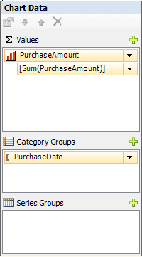
Figure 3
Expand the size of the chart two or three times. Save the report and navigate to the Preview tab to run the report. It should look as shown in Figure 4.
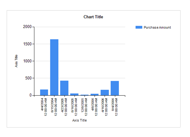
Figure 4
This report shows total sales by purchase date, but what if it needed instead to show the sales by date for different types of purchase, such as online purchases, versus in-store purchases, and so on. You can achieve this by adding the PurchaseType field as a Series Group. For every field in the Values area, we’d see a series of bars, each one representing a distinct value that exists in the Series Group field. So, for example, if the PurchaseType field contains three distinct types of purchase, then you’ll see three series for each field in the Values area.
In the Series Groups section of the chart’s data properties, click the plus sign and add PurchaseType. Preview the report again, and you should see the data displayed based on the type of purchase.
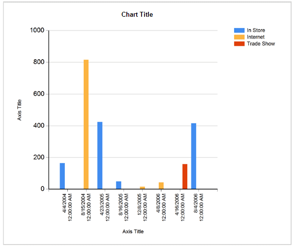
Figure 5
Formatting the Chart
You now have a chart, but, there is still work to do in order to get it into a nice format. For a start, the date format does not look good, so fix that first. On the Design tab of the report, right-click the text area along the bottom of the chart that says “Purchase date A” and bring up the Horizontal Axis Properties dialog. Select the Number option from the left menu, and then the Date category. Select the appropriate date format and click OK. You can make the same type of change to the vertical axis if needed, for example formatting it as currency. Often the numbers on the vertical axis are very large and it might help to display the values as thousands, for example.
Modify the title at the top of the chart and then remove or modify the axis titles. If you wish to change the sort order of the Category Group field, click the dropdown box next to the category, select the Category Group Properties and navigate to the Sorting section. To change the color of the bars, right-click the one of them to get to the properties. After tweaking the properties, my report looks like Figure 6.
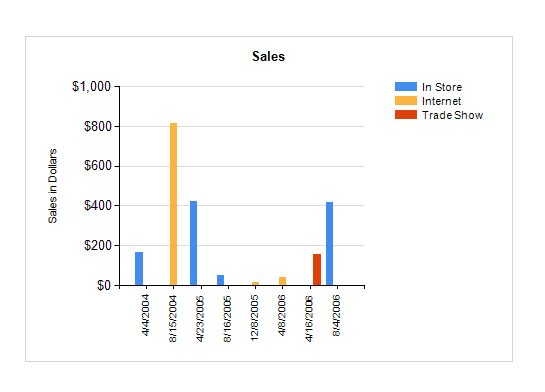
Figure 6
Chart types
As noted earlier, the chart control can produce a variety of the different chart types. To switch to a different type, simply right-click on the chart (in the Design tab) and use the Change Chart Type option.
First, remove the Series Group (right click PurchaseType and select Remove Series Group) and try switching to a Smooth Line chart, the second of the line chart types. Right-click the series line and choose Series Properties. On the Series Data page, select [Sum(PurchaseAmount)] in the Tooltip dropdown box. On the Markers page, change the Marker Type to Circle and click OK.
Now when you run the report, hovering the mouse over a data point should reveal its value as a tooltip. You can format the ToolTip value by changing the Tooltip property to an expression that uses the FormatCurrency function: FormatCurrency(Sum(Fields!PurchaseAmount.Value)). Figure 7 shows how the report should look.
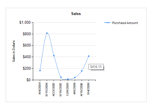
Figure 7
Indicators
So far you have looked at charts to compare data over time, or by some other measure. You can also add visual elements to regular report sections. One visual element you can add is called an Indicator, which is generally used to provide a simple, visual signal of success or failure. For example, an indicator could show an upward arrow if a goal is met, a horizontal arrow if it is close, and a downward arrow if the goals was missed by a wide margin.
Create a new report called Indicators.rdl with the same data source and dataset (Listing 1) as the MyChart report. Drag a table control into the report design area, and populate it with the PurchaseDate, CustomerName and PurchaseAmount fields. Format the report (highlight the header row and hit F4 to set the font and background color), then and add a new column to the right, as shown in Figure 8.
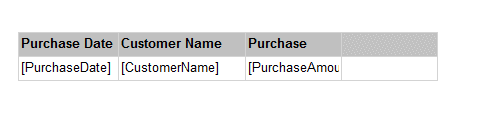
Figure 8
Drag an Indicator control to the empty cell and use the automatic Select Indicator Type dialog box to choose one of the indicator types. It is a good practice to select an indicator that changes shape, as well as color, depending on the value. If the shapes are identical, then the colors are lost when printed on a non-color printer. There are also many color blind people who can’t distinguish all colors.
The Indicator can be set to one value, the one that you want to measure. Click the indicator control to open the Gauge Data window and select PurchaseAmount as the indicator value. SSRS will automatically apply a Sum expression.
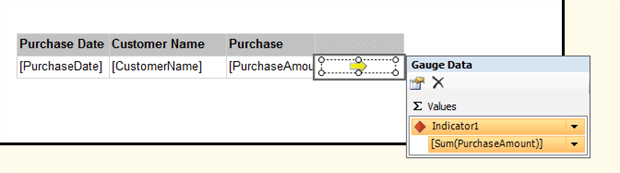
Figure 9
Preview the report and you should see an indicator, with the default properties, revealing at a glance the low, mid-range and high value sales, as shown in Figure 10.
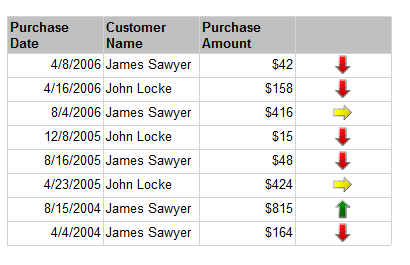
Figure 10
By default, the indicator is based on percentages and distributed by thirds, but the properties of the indicator are very customizable. On the design view, right-click the indicator, select Indicator Properties, click Values and States where you can customize the values or percentages that determines which indicator to display. Figure 11 shows the default properties.
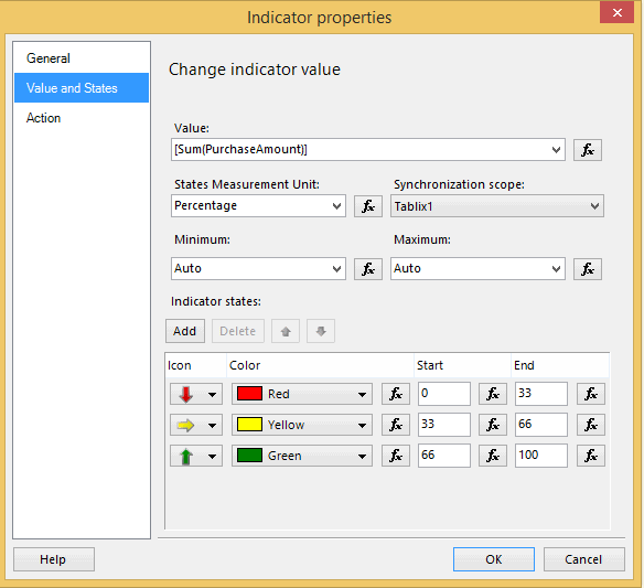
Figure 11
You can alter the percent ranges, switch to specific values instead, modify the colors and indicators, or even add additional indicators for more ranges.
Gauges
The gauge is a slightly more complex control that compares the data to a set goal. Again, though, its basic purpose is to allow a manager to see quickly the progress towards a given goal.
Say you’re asked to provide a manager with a report that will tell him or her quickly whether or not the team is on track to meet a yearly sales target. Create a new report called Gauge with the same ReportDb data source. The data set just needs to include the field to measure, in this case the SUM([PurchaseAmount]), broken down by year, so use the query in Listing 2.
|
1 2 3 4 |
SELECT YEAR([PurchaseDate]) AS PurchaseYear , SUM([PurchaseAmount]) AS Amt FROM [Purchase] GROUP BY YEAR(PurchaseDate) |
Listing 2
Add a table control to the report containing both of the fields. In the third data cell, drag in a gauge control. When prompted to select a gauge type, choose the first Linear gauge. Expand the width and height of the cell containing the gauge and format the report so that it looks similar to Figure 12.
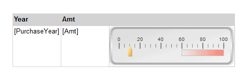
Figure 12
At a minimum, you must set the value to measure, so click on the gauge to open the Gauge Data window and select Amt from the list. Once again, SSRS applies the SUM aggregate function automatically.
Right now, the gauge resembles a Celsius thermometer at 10 degrees. If you run the report now, all of the values will be at 100 since the amounts are all over 100, as shown in Figure 13.
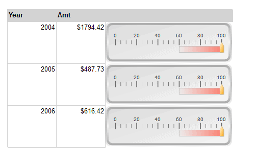
Figure 13
To alter the scale and the range (the red area), return to the Design tab. Right-click the range to bring up the Linear Scale Range Properties dialog box. Change the Start range scale value to 0 and End range at scale value to 1000. On the Fill properties, change the Color to Red and the Secondary Color to Green. Click OK.
Next, right-click on the scale and bring up the Linear Scale Properties dialog box. On the General tab, set the Maximum value to 1000. Click OK and now preview the report as shown in Figure 14.
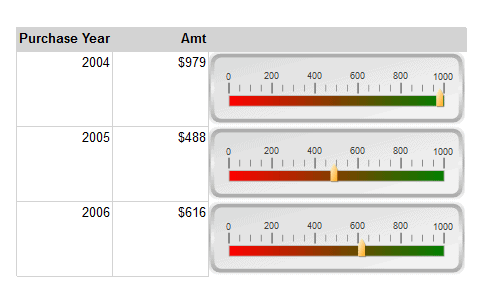
Figure 14
You can also add a gauge control to the report, outside of the table. In this case, the gauge will display the total aggregate value across the entire data set, in this case the total purchase amount over all years.
Add a gauge control to the report area, and select the default type. Set the properties in a similar way as the previous example, but use 3000 for the maximum value of the scale and range. When you preview the report, the gauge should look similar to Figure 15.
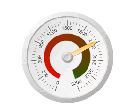
Figure 15
Data bars and Sparklines
Data bars and Sparklines allow you to add visual detail to a grouping level within a report. For example, say you want to add a visual element to the report that indicates the trend of the sales for each month. This is a perfect use case for the sparkline. If you also want a visual way to see the sales broken down by categories then you can use a data bar.
Create a new report called SparklineDatabar. Listing 3 show the query for the report.
|
1 2 3 4 5 6 7 |
SELECT YEAR([PurchaseDate]) AS PurchaseYear , SUM([PurchaseAmount]) AS Amt , MONTH(PurchaseDate) AS PurchaseMonth , PurchaseType FROM [Purchase] GROUP BY YEAR(PurchaseDate) , MONTH(PurchaseDate) , PurchaseType |
Listing 3
Drag a table to the report and add the Amt. Right-click on Amt, select Add Group | Row Group | Parent Group, group by PurchaseYear and check Add group header. Remove one of the empty columns. At this point, the report should similar to Figure 16.
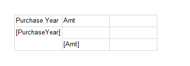
Figure 16
Drag a data bar control to the cell at the intersection of the third column and second row. Select the default type and click OK. Click the data bar to open up the Chart Data window which looks just like the window used in the regular chart earlier in the article. Select Amt for the summary value and PurchaseType for the category group. The properties should look like Figure 17.
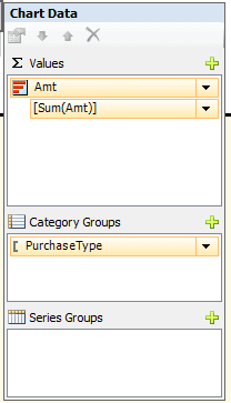
Figure 17
The data bar control is essentially a small version of the chart control. Because it sits inside a cell, you cannot read the values or category. If the user of the report would like to see the values, you can add a tooltip. To do this, click twice in the cell with the data bar to select the bars. Right-click and select Series Properties. Click the Fx button next to the Tooltip property. Enter this expression:
|
1 |
=Fields!PurchaseType.Value & ": " & FormatCurrency(Fields!Amt.Value,0) |
Click OK twice to close both dialogs and then preview the report. Remember to mouse over the bars to see the tooltip. The report should look like Figure 18.
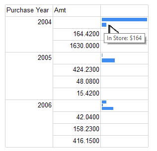
Figure 18
Now back in the Design tab, add another column to the table. This time drag in a sparkline control to the cell next to the data bar and choose the first Line type. This time the category group should be PurchaseMonth. The data bar showed how the data was broken down by type of sale, but the sparkline will show how the data is broken down by month. Figure 19 shows how the properties should be set.
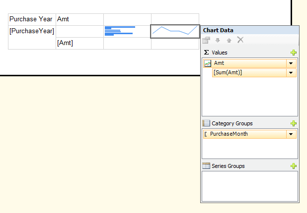
Figure 19
The tooltip expression for the sparkline’s Series Properties should be as follows:
|
1 2 |
=MonthName(Fields!PurchaseMonth.Value) & ": " & FormatCurrency(Fields!Amt.Value,0) |
Change the Marker Type to Square. Preview the report. It should look like Figure 20.
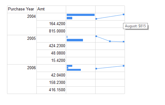
Figure 20
Maps
The final type of visualization is probably the most interesting. You can add maps to your reports to display data geographically. In this section, you will just set up a simple map that shows the location of the sales, but the world is your limit here (pun intended).
Add a new report called Map with a dataset called MapData, defined by the query in Listing 4.
|
1 2 3 4 5 6 7 8 9 10 11 |
SELECT Purchase.PurchaseID , Purchase.CustomerID , Purchase.PurchaseDate , Purchase.PurchaseType , ISNULL(Purchase.PurchaseAmount, 0) AS Amt , CASE WHEN PurchaseType IS NULL THEN 0 ELSE 1 END AS Sale , State FROM Customer LEFT JOIN Purchase ON Purchase.CustomerID = Customer.CustomerID |
Listing 4
Add a map control from the Toolbox. When you do, a wizard appears. On the first page, you select the source of spatial data. You can select the built-in maps from the Map Gallery, an ESRI shape file, or spatial data from SQL Server. Select the simplest choice, the Map Gallery and USA by State Exploded. Click Next.
The following screen allows you to zoom in and crop. Youcan also add a Bing Maps layer. The Bing Maps layer is really cool, but it can distract from the meaning of the data. For now, accept the defaults on this screen and click Next.
On the Choose map visualization page, youselect the type of map, Basic, Color Analytical or Bubble. Select the Color Analytical Map and click Next. The next page is where you map a dataset to the map. Select the MapData dataset.
On the Specify the match fields for special and analytical data page, you will link a field from the map itself to a field in the dataset. The data in the middle section is from the map. The data in the lowest section is your data. You need to map the STUSPS field from the Spatial data section to the State field in the dataset, so check the Match Fields checkbox next to STUPS, and select the State field in the Analytical dataset fields section, as shown in Figure 21.
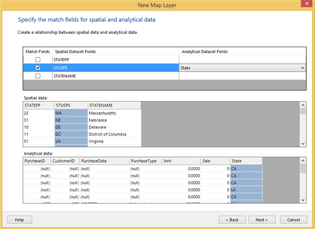
Figure 21
Click Next. On the Choose color theme and data visualization page you will set the color properties and link the colors to a field in the data. In the Field to visualize, select SUM([Amt]). The Color rule is set so that smaller values are green and larger values are red, the opposite of what you need to see. Switch the order to Red-Yellow-Green. Click Finish and preview the report. It should look like Figure 22.
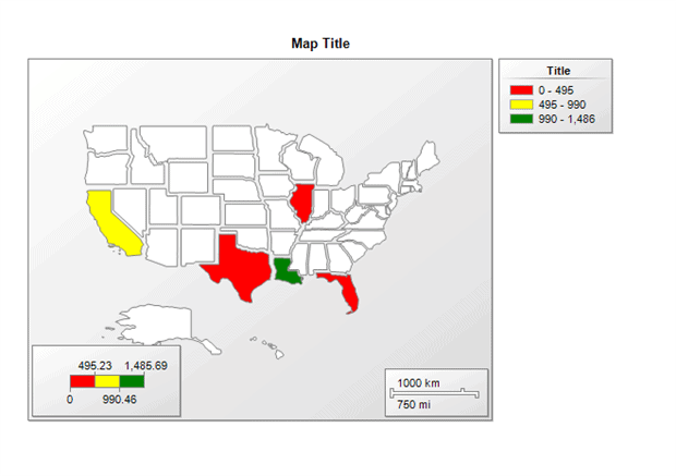
Figure 22
Wrap up
I hope this article has given you some insight into the visual controls. Between the visual controls’ rich features and SSRS’s ability to set nearly every property with an expression, you can see that Microsoft has delivered an extremely powerful and user-friendly set of visual features in this reporting tool.
Stay tuned for Part 4 of this article series, which will peel back the layers on RDL (Report Definition Language) and take a look at Report Builder.


Load comments