
As DBAs, there are many things we need to worry about. In my last article, Planning for Disaster, I covered the importance of a pessimistic mindset when devising a disaster recovery plan. In this one, I’ll tackle perhaps the biggest headache for a DBA: a slow and unreliable storage system.
I’ll cover a number of tactics and methods employed by experienced DBAs to ensure that their storage systems perform adequately, and are capable of handling peak load requirements. The next article will look at storage reliability and integrity.
Performance-Centric vs. Capacity-Centric Designs
It’s very common to hear customers complain about the quoted cost and delivery time of enterprise storage. How much!? I can walk down to Best Buy and purchase a Terabyte drive for $100 and have it ready in 30 minutes! Of course, it’s more complicated than that. As DBAs we need to consider backups, performance, manageability and numerous other factors, mostly absent in the consumer space. That being said, it still surprises me how often a capacity-centric storage design approach is used by DBAs today.
Consider a request for a new 500GB database. How many hard disks do we need to fulfil that request? A capacity-centric approach would use a single 640GB disk. Nice and easy, except we have no idea how the system will perform, let alone issues surrounding backups and fault tolerance. Using a performance-centric approach, we’ll look at this in a completely different manner. Before we even consider the size requirements, we look at the throughput requirements and calculate the number of disks using simple division based on the throughput of each disk. More on that shortly…
A fundamental performance tuning task is to identify the biggest bottleneck. Once located, the bottleneck can be removed, or at least alleviated, in order to increase throughput to an acceptable level. While it’s true that the biggest performance gains can often be realized through good application design, running on sub-optimal hardware makes the performance tuning process much more difficult. Hard disks, as the slowest hardware component, deserve special consideration when optimizing the hardware platform on which SQL Server runs.
Hard Disks and Seek Time
Conventional hard disks are mechanical components; that is, they’re comprised of moving parts. Circular platters spin and disk arms move in and out from the centre of the platters, thus enabling all parts of the disk to be read. The time it takes to physically move the disk heads (on the end of the disk arm) to the correct position is known as the seek time. The seek time in combination with other measurements such as rotational time and transfer time, determines the overall speed of the drive.
The seek time for any given disk is determined by how far away from the required data the disk heads are at the time of the read/write request. In typical OnLine Transaction Processing (OLTP) databases, the read/write activity is largely random; each transaction will likely require data from a different part of the disk. It follows that in most OLTP applications, hard disks will spend most of their time seeking data, therefore, the seek time of the disk is a crucial bottleneck.
There are limits to how fast a disk can spin and how fast disk heads can move and, arguably, we reached that limit many years ago. What should be obvious by now is that in order to overcome these physical limits, we need to use multiple disks, therefore reducing the effects of seek/spin time. Enter RAID. In addition to providing protection against data loss through the redundant storage of data on multiple disks, RAID partitions stripe data across many disks. This increases performance by avoiding the bottlenecks of a single disk. The next question is how many disks do we need?
How many Disks?
In answering this question we need to consider two important measurements. Firstly, the number of reads and writes we expect our database to perform per second, and secondly, the IO per second (IOPS) rating of each disk. Expressed as a formula, we have:
|
1 |
Required # Disks = (Reads/sec + (Writes/sec * RAID adjuster)) / Disk IOPS |
You’ll note that we’ve multiplied writes/sec by “RAID Adjuster”. RAID disk systems write the same piece of data multiple times in order to provide fault tolerance against disk failure. The RAID level chosen determines the multiplier factor. For example, a RAID 1 (or 10) array duplicates each write and so the RAID multiplier is 2. RAID 5, discussed later in this article, has a higher write overhead in maintaining parity across the disks, and therefore has a higher multiplier value.
The next question is: how many reads and writes per second does the database perform? There are a few ways to answer that question. For existing production systems, we can measure it using the Windows Performance Monitor tool. For systems in development, we can measure the reads/writes per transaction, and then multiply this value by the peak number of transactions per second that we expect the system to endure. I emphasize peak transactions, because it’s important to plan for maximum expected load.
Say, for example, we’re designing a RAID 10 system. The individual disks are capable of 150 IOPS and the system as a whole is expected to handle 1200 reads per second and 400 writes per second. We can calculate the number of disks required as follows:
|
1 |
Required # Disks = (1200 + (400 * 2)) / 150 = ~13 DISKS |
What about capacity? We haven’t even considered that yet, and deliberately so. Assuming we’re using 72GB disks, 13 of them will give us a capacity of about 936GB, or just over 450GB usable space after allowing for duplicate writes under RAID. If our estimated database size is only 100GB, then we have ~ 22% utilization to ensure we can meet peak throughput demand. In summary, this is the performance-centric approach.
Determining the number of disks required is only one (albeit very important) aspect of designing a storage system. The other crucial design point is ensuring that the I/O bus is capable of handling the IO throughput. The more disks we have, the higher the potential throughput requirements and we need to be careful to ensure we don’t saturate the IO bus.
All Aboard the IO Bus!
To illustrate IO bus saturation, let’s consider a simple example. A 1GB fiber channel is capable of handling about 90 MB/Sec of throughput. Assuming each disk it services is capable of 150 IOPS (of 8K each), that’s a total of 1.2 MB/Sec, which means that the channel is capable of handling up to 75 disks. Any more than that and we have channel saturation, meaning we need more channels, higher channel throughput capabilities, or both.
The other crucial consideration here is the type of IO we’re performing. In the above calculation of 150*8K IOPS, we assumed a random/OLTP type workload. In reporting/OLAP environments, we’ll have a lot more sequential IO consisting of, for example, large table scans during data warehouse loads. In such cases, the IO throughput requirements are a lot higher. Depending on the disk, the maximum MB/Sec will vary, but let’s assume 40 MB/Sec. It only takes three of those disks to produce 120 MB/Sec, leading to saturation of our 1GB fiber channel.
In general, OLTP systems feature lots of disks to overcome latency issues, and OLAP systems feature lots of channels to handle peak throughput demands. It’s important that we consider both IOPS, to calculate the number of disks we need, and the IO type, to ensure the IO bus is capable of handling the throughput. But what about SANs?
Storage Area Networks (SAN)
Up to now I’ve made no mention of SANs. Regardless of the storage method, be it SAN or Direct Attached Storage (DAS), the principles of I/O throughput and striping data across multiple disks remains the same. However, depending on the SAN vendor, there are many different techniques used to construct a logical disk partition (LUN) for use by SQL Server, and some of them, such as concatenating disks rather than striping, are simply not appropriate.
The scope of this article does not allow for a detailed look at SAN design, but suffice to say that it’s very important for a DBA to be involved in the process as early as possible. A DBA cannot simply abdicate their IO design responsibilities on the assumption that the default SAN design will suffice. SQL Server, despite what many SAN administrators may tell you, is special, and time spent up front getting the SAN design right will save a huge amount of pain later on.
One of the challenging aspects of performance tuning SQL Server SAN storage (or any storage for that matter) is defining what is fast and what is slow. One DBA’s definition of slow may be incredibly fast to another, so measuring performance, and having a performance baseline to give your measurements meaning, is crucial. Enter SQLIO.
SQLIO
Available from Microsoft as a free download, SQLIO is a tool used to measure various aspects of a storage system, such as latency, IOPS and throughput. Despite the name, SQLIO does not have any direct link to SQL Server. It’s best used to tune the storage system before SQL Server is installed, therefore avoiding costly and time-consuming production IO reconfigurations, when we discover our storage was never installed correctly to begin with!
SQLIO is used to obtain raw numbers useful for comparing the performance of systems with similar specifications. For example, if the SAN vendor tells you that you should expect 10,000 IOPS in a given configuration, and SQLIO records 2000, then it’s a fair bet that something is either not configured correctly, there are driver/firmware issues, or the vendor was lying! Either way, this type of testing is essential in ensuring optimal storage configuration, and for validating proposed changes to an existing system.
=”margin-left:.5in”>
Let’s move now from hardware to SQL Server database file configuration, and look at five common IO myths & mistakes.
Common SQL Server IO Configuration Myths & Mistakes
There are many things we can do wrong, as DBAs, when it comes to IO performance, and there are just as many myths. Listed here are five of the most common mistakes.
- Mixing transaction logs & data on the same disk(s);
Unlike the random read/write patterns of a database’s data file, the transaction log is used in a sequential manner, i.e. transactions are written to disk one after the other. A common design mistake is to put transaction logs on the same disk/s as the data files. This leads to a situation where the disk heads are subject to the conflicting requirements of random and sequential IO. By placing the transaction log on a dedicated disk, the disk heads can stay in position, writing sequentially. For very high throughput applications, this is crucial in avoiding transaction bottlenecks.
- Using multiple log files
Unlike using multiple data files (discussed next), there is no performance benefit to be gained from using multiple transaction log files. Better transaction log performance comes from disk isolation, as discussed in the previous point, using faster disks, ensuring the log is sized appropriately for initial and ongoing requirements, and avoiding frequent autogrow events along with the subsequent fragmentation this can cause.
- Using one data file per CPU
A common database performance tuning recommendation is to use one data file per CPU to boost IO performance. As Paul Randal (blog | twitter) explains in this post, this recommendation does not (usually) make sense for user databases, but it does make sense for the tempdb database, in overcoming allocation bitmap contention. Note that this recommendation is not to be confused with using multiple data files across several filegroups, in order to control the placement of database objects across distinct IO paths. That does make sense, but only if you know your application’s IO profile well enough and have verified the performance improvements. Unless you’re in that category, it’s often a better approach to use a single filegroup spread across as many disks as possible, in order to obtain the best striping performance.
- Using the default partition alignment
As Jimmy May and Denny Lee explain in this Microsoft Whitepaper, prior to Windows Server 2008 disk partitions created using the default settings are unaligned, meaning that multiple IOs are required to read every nth cluster. If you align the partition, at creation time, this corrects the multi IO situation and may result in a staggering increase in IO performance. This is a classic example of how such a basic (and simple) configuration step can have a massive impact on performance.
Using RAID-5
The conventional wisdom among database professionals is that RAID-5 is evil and should be avoided regardless of the situation. The primary issue with RAID-5 is that in addition to a parity calculation, each logical write requires many physical writes. The performance effects of this are most keenly felt on systems with a high write percentage, and are made worse in cases where there is not enough RAM. It follows that on systems with a low write percentage, and on those with sufficient memory, RAID-5 may not be such a performance killer as many make it out to be. The bottom line is that, depending on the IO profile and the storage implementation, the performance difference between a RAID-5 and a RAID-10 array may not be discernable at all, and the extra costs of a RAID-10 array may be better spent elsewhere.
Before we finish this article, it would be remiss of me to skip over the possibilities offered by Solid State Disks.
Solid State Disks
Earlier in this article, we spoke of a hard drive as a mechanical object with moving parts. That, of course, applied to a conventional magnetic hard drive, with spinning platters, as opposed to a flash memory-based solid state disk (SSD). SSDs have been around in the consumer space for quite some time and, in recent years, we’ve also seen the emergence of SSDs in the enterprise space.
From a database perspective, the main benefit of SSDs is that there are no moving parts. As a result, seek time, whereby a disk arm has to swing over a spinning platter to read data, is largely eliminated. This means that random data access can be many, many times faster in an SSD implementation. In OLTP applications, using traditional magnetic hard drives, I’ve advised the use of multiple disks to overcome the effects of seek time. However, if seek time on SSDs is no longer an issue, what does this mean for the future of SQL Server IO storage systems?
With dramatically reduced seek time comes an increasing likelihood of bus saturation. Take the SATA bus, for example. It has a throughput capacity of up to 300 MB/Sec. A single decent SSD drive will easily overwhelm that bus, meaning that the bottleneck in an SSD system immediately shifts from disks to the bus and makes the bus configuration an important part of deriving maximum benefit from an SSD system.
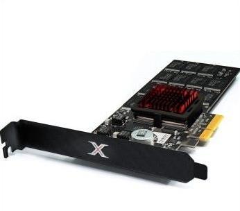
A recent development in SSD technology, used to get around bus saturation, is to connect the SSDs directly to the PCI express (PCI-e) bus inside the server, which has a throughput of up to 16 GB/Sec. The leading example of this implementation is the ioDrive from Fusion-io. There have been some truly staggering figures emerge from these implementations, with FusionIO’s website claiming up to 1.5 GB/Sec throughput and ~185,000 IOPS per drive. Scaled linearly, four such drives could therefore achieve up to 6 GB/Sec throughput and ~750,000 IOPS.
However, before we get too carried away by these numbers, there are a few important points to note about SSD technology. Firstly, write performance tends to be much lower than read so, depending on the IO profile of the application, performance will obviously vary. Secondly, the PCI express implementations have a number of particular limitations:
- PCI express cards don’t easily fit into blade servers
- PCI express cards are a single-server implementation, so they cannot be used as shared storage for clustering SQL Server instances.
- There’s no hardware based RAID solution for SSDs, so we’re forced to use software-based RAID.
- There’s obviously no hot swap capability to handle failed drives.
With these limitations, SSD drives are not about to replace traditional SAN storage anytime soon. However, for single server solutions that may not require maximum high-availability they do offer an incredible performance boost for dramatically less money than a traditional SAN solution.
Any discussion on database storage is not complete without significant attention to integrity and reliability, and such matters will be the focus of the next article.
Load comments