
Hi Folks, I’m going to start a new series of three articles about Window functions, starting off by explaining what they are, and how they are used to provide details of an aggregation.
Window functions
Window functions belong to a type of function known as a ‘set function’, which means a function that applies to a set of rows. The word ‘window’ is used to refer to the set of rows that the function works on.
Windowing functions were added to the standard SQL:2003 that is managed by the ISO and it was specified in more detail in SQL:2008 For some time, other DBMSs such as Oracle, Sybase and DB2 have had support for window functions. Even the open source RDBMS PostgreSQL has a full implementation. SQL Server has had only a partial implementation up to now, but it is coming in SQL 2012.
One of the most important benefits of window functions is that we can access the detail of the rows from an aggregation. To see an example, let’s first suppose we have this table and data:
|
1 2 3 4 5 6 7 8 9 10 11 12 13 |
USE tempdb GO IF OBJECT_ID('TestAggregation') IS NOT NULL DROP TABLE TestAggregation GO CREATE TABLE TestAggregation (ID INT, Value Numeric(18,2)) GO INSERT INTO TestAggregation (ID, Value) VALUES(1, 50.3), (1, 123.3), (1, 132.9), (2, 50.3), (2, 123.3), (2, 132.9), (2, 88.9), (3, 50.3), (3, 123.3); GO |
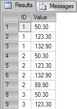
This is what the data looks like:
|
1 |
SELECT * FROM TestAggregation |
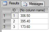
If we sum the column Value grouping by ID, by using a conventional GROUP BY, we would have the following query and result:
|
1 2 3 |
SELECT ID, SUM(Value) FROM TestAggregation GROUP BY ID; |
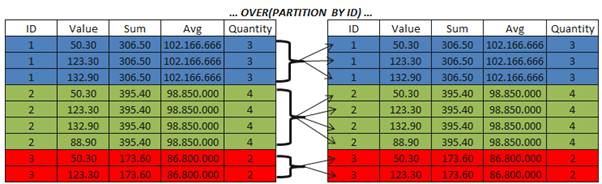
Here we can see a sample of the partitions of rows, or sets that the SUM aggregation function is working on.
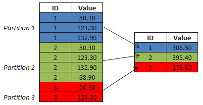
In the blue we have partition 1, green as partition 2 and red as partition 3. Because we applied the aggregation function in the column value, grouping the results by ID, we the lose the details of the data. In this case the details are the values of the columns of the rows in the partitions 1, 2 and 3.
Let’s suppose I need to write a query to return the total value of sales, the average value of sales and the quantity of sales for each ID, and still return the actual values of the rows, then we might think that we could use something like this to return this data:
|
1 2 3 4 5 6 |
SELECT ID, Value, SUM(Value) AS "Sum" AVG(Value) AS "Avg" COUNT(Value) AS "Quantity" FROM TestAggregation GROUP BY ID; |
Msg 8120, Level 16, State 1, Line 2
Column ‘TestAggregation.Value’ is invalid in the select list because it is not contained in either an aggregate function or the GROUP BY clause.
Unfortunately it is against the way that aggregations work. If you group by something, then you lose access to the details.
A very commonly used alternative is to write every aggregation into a subquery, and then correlate with the main query using a join, something like:
|
1 2 3 4 5 6 7 8 9 10 11 12 13 14 15 16 17 18 |
SELECT TestAggregation.ID, TestAggregation.Value, TabSum."Sum" TabAvg."Avg" TabCount."Quantity" FROM TestAggregation INNER JOIN (SELECT ID, SUM(Value) AS "Sum" FROM TestAggregation GROUP BY ID) AS TabSum ON TabSum.ID = TestAggregation.ID INNER JOIN (SELECT ID, AVG(Value) AS "Avg" FROM TestAggregation GROUP BY ID) AS TabAvg ON TabAvg.ID = TestAggregation.ID INNER JOIN (SELECT ID, COUNT(Value) AS "Quantity" FROM TestAggregation GROUP BY ID) AS TabCount ON TabCount.ID = TestAggregation.ID |
But a neater and faster solution is this…
|
1 2 3 4 5 6 7 8 9 10 11 12 13 14 15 |
SELECT TestAggregation.ID, TestAggregation.Value, AggregatedValues.[Sum], AggregatedValues.[Avg], AggregatedValues.Quantity FROM TestAggregation INNER JOIN ( SELECT ID, SUM(Value) AS "Sum" AVG(Value) AS "Avg" COUNT(Value) AS "Quantity" FROM TestAggregation GROUP BY ID) AggregatedValues ON AggregatedValues.ID=TestAggregation.ID |
A very elegant alternative is to use the clause OVER() implemented in the aggregation functions, it allow-us to access the details of the rows that have been aggregated.
For instance we could try to get the result we want with this …
|
1 2 3 4 5 |
SELECT ID, Value, SUM(Value) OVER() AS "Sum" AVG(Value) OVER() AS "Avg" COUNT(Value) OVER() AS "Quantity" FROM TestAggregation |
…but, with this query, we didn’t return the expected results. In fact, we returned the aggregate values for the entire table rather than for each ID. Using the clause OVER() with the aggregation function (SUM, AVG and COUNT) we have accessed the details of the grouped data along with a total aggregation of the data, but, in In fact, we want the aggregates for the data grouped by ID. To do this, we should use the clause PARTITION BY clause. For instance:
|
1 2 3 4 5 6 |
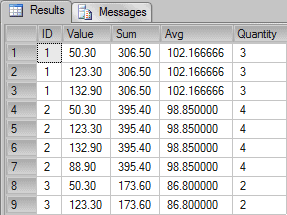
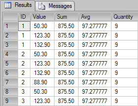
SELECT ID, Value, SUM(Value) OVER(PARTITION BY ID) AS "Sum" AVG(Value) OVER(PARTITION BY ID) AS "Avg" COUNT(Value) OVER(PARTITION BY ID) AS "Quantity" FROM TestAggregation |
Now we can see the same results as in the subquery alternative, but with a much more simple and elegant code.
In the following picture we can see that even the results are grouped by ID we can see access the details of the aggregated partitions through the clause OVER and PARTITION BY.
Set based thinking
It can get tedious to hear about this set base thing, but in fact it’s not so easy to think set based. Sometimes it’s very hard to find a set based solution to a query we have. Window Functions give us more set-based solutions to awkward problems.
The main point of windowing functions it’s that they were created to work with a set. SQL Server never was good on processing queries row by row, that’s why you always hearing that ‘cursors are evil’, and are ‘not good for performance’, ‘you should avoid them’ and so on. SQL Server was not built to work row by row.
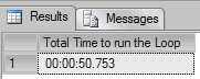
Let’s illustrate this. SQL Server takes an average of 50 seconds to run a loop of 1 hundred million times against 100 milliseconds of a Win32 app.
|
1 2 3 4 5 6 7 |
DECLARE @i INT = 0, @Time Time(3) = GETDATE() WHILE @i < 100000000 BEGIN SET @i += 1; END SELECT CONVERT(Time(3), GETDATE() - @Time) AS "Total Time to run the Loop" |
Delphi Code:
|
1 2 3 4 5 6 7 8 9 10 11 |
PROCEDURE TForm1.Button1Click(Sender: TObject); Var i : Integer; Tempo : TDateTime; BEGIN i := 0; Tempo := Now(); WHILE i < 100000000 do BEGIN inc(i); END; |
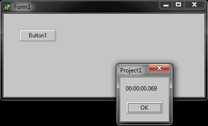
Of course it is an unfair comparison. The compiler of a win32 application is totally different from SQL Server, what I wanted to show here is the fact that SQL Server was not supposed to run row by row.
I once was in London doing training with my colleague Itzik Ben-Gan when I remember he said: “There is no row-by-row code that you cannot run an equivalent set-based version, the problem is that you didn’t figured out how to do it”. Yes it’s a heavy phrase but, who could tell Itzik that this is not true? Not I!
Window functions on SQL Server 2005 and 2008
Since SQL Server 2005 we have had support for some window functions, they are: ROW_NUMBER, RANK, DENSE_RANK and NTILE.
In this first article we’ll review how these functions works, and how they can help-us to write better and efficient set-based codes.
Test database
To test the functions we’ll use a table called Tab1. The code to create the table is the following:
|
1 2 3 4 5 6 7 8 9 10 |
USE TempDB GO IF OBJECT_ID('Tab1') IS NOT NULL DROP TABLE Tab1 GO CREATE TABLE Tab1 (Col1 INT) GO INSERT INTO Tab1 VALUES(5), (5), (3) , (1) GO |
Row_Number()
The ROW_NUMBER function is used to generate a sequence of numbers based in a set in a specific order, in easy words, it returns the sequence number of each row inside a set in the order that you specify.
For instance:
|
1 2 3 4 |
-- RowNumber SELECT Col1, ROW_NUMBER() OVER(ORDER BY Col1 DESC) AS "ROW_NUMBER()" FROM Tab1 |
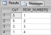
The column called “ROW_NUMBER()” is one of a series of numbers created in the order of Col1 descending. The clause OVER(ORDER BY Col1 DESC) is used to specify the order of the sequence for which the number should be created. It is necessary because rows in a relational table have no ‘natural’ order.
Rank() & Dense_Rank()
Return the position in a ranking for each row inside a partition. The ranking is calculated by 1 plus the number of previews rows.
It’s important to mention that the function RANK returns the result with a GAP after a tie, whereas the function DENSE_RANK doesn’t. To understand this better, let’s see some samples.
|
1 2 3 4 5 6 7 8 |
-- Rank SELECT Col1, RANK() OVER(ORDER BY Col1 DESC) AS "RANK()" FROM Tab1 GO -- Dense_Rank SELECT Col1, DENSE_RANK() OVER(ORDER BY Col1 DESC) AS "DENSE_RANK" FROM Tab1 |
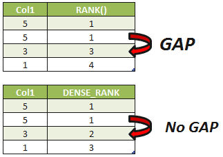
Notice that in the RANK result, we have the values 1,1,3 and 4. The value Col1 = “5” is duplicated so any ordering will produce a ‘tie’ for position between them. They have the same position in the rank, but, when the ordinal position for the value 3 is calculated, this position isn’t 2 because the position 2 was already used for the value 5, in this case the an GAP is generated and the function returns the next value for the tank, in this case the value 3.
NTILE()
The NTILE function is used for calculating summary statistics. It distributes the rows within an ordered partition into a specified number of “buckets” or groups. The groups are numbered, starting at one. For each row, NTILE returns the number of the group to which the row belongs. It makes it easy to calculate n-tile distributions such as percentiles.
Let’s see a sample:
|
1 2 3 4 |
-- NTILE SELECT Col1, NTILE(3) OVER(ORDER BY Col1 DESC) AS "NTILE(3)" FROM Tab1 |
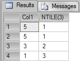
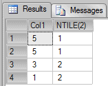
In the result above we can see that 4 rows were divided by 3 it’s 1, the remaining row is added in the initial group. Let’s see another sample without remained rows.
|
1 2 3 4 |
-- NTILE SELECT Col1, NTILE(2) OVER(ORDER BY Col1 DESC) AS "NTILE(2)" FROM Tab1 |
It is good practice to order on a unique key, ensure that there are more buckets than rows, and to have an equal number of rows in each bucket
The Power of Window functions
Now let’s see some examples where window functions could be used to return some complex queries.
Example 1
Let’s suppose I need to write a query to return those employees that receive more than his department’s average.
Let’s start by creating two sample tables called Departamentos (departments in Portuguese) and Funcionarios (employees in Portuguese):
|
1 2 3 4 5 6 7 8 9 10 11 12 13 14 15 16 17 18 19 20 21 22 23 24 25 |
IF OBJECT_ID('Departamentos') IS NOT NULL DROP TABLE Departamentos GO CREATE TABLE Departamentos (ID INT IDENTITY(1,1) PRIMARY KEY, Nome_Dep VARCHAR(200)) GO INSERT INTO Departamentos(Nome_Dep) VALUES('Vendas'), ('TI'), ('Recursos Humanos') GO IF OBJECT_ID('Funcionarios') IS NOT NULL DROP TABLE Funcionarios GO CREATE TABLE Funcionarios (ID INT IDENTITY(1,1) PRIMARY KEY, ID_Dep INT, Nome VARCHAR(200), Salario Numeric(18,2)) GO INSERT INTO Funcionarios (ID_Dep, Nome, Salario) VALUES(1, 'Fabiano', 2000), (1, 'Amorim', 2500), (1, 'Diego', 9000), (2, 'Felipe', 2000), (2, 'Ferreira', 2500), (2, 'Nogare', 11999), (3, 'Laerte', 5000), (3, 'Luciano', 23500), (3, 'Zavaschi', 13999) GO |
This is what the data looks like:
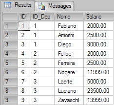
To write this query I could do something like this:
|
1 2 3 4 5 6 7 8 |
SELECT Departamentos.Nome_Dep, Funcionarios.Nome AS Funcionario, Funcionarios.Salario, AVG(Funcionarios.Salario) OVER(PARTITION BY Departamentos.Nome_Dep) "Média por Departamento" Salario - AVG(Funcionarios.Salario) OVER(PARTITION BY Departamentos.Nome_Dep) "Diferença de Salário" FROM Funcionarios INNER JOIN Departamentos ON Funcionarios.ID_Dep = Departamentos.ID ORDER BY 5 DESC |
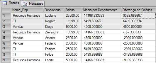
As we can see, the employees Luciano, Nogare and Diego are receiving much more than the average of their department.
Using the OVER clause, I was able to partition the data per each department, and then I could access the average with the details of the salary.
You can avoid using window functions by using a query like this.
|
1 2 3 4 5 6 7 8 9 10 11 12 13 14 |
SELECT Departamentos.Nome_Dep, Funcionarios.Nome AS Funcionario, Funcionarios.Salario, [Média por Departamento], Salario - [Média por Departamento] AS [Diferença de Salário] FROM Funcionarios INNER JOIN Departamentos ON Funcionarios.ID_Dep = Departamentos.ID INNER JOIN ( SELECT ID_Dep, AVG(Funcionarios.Salario) AS [Média por Departamento] FROM Funcionarios GROUP BY ID_Dep)[Média] ON [Média].ID_Dep=Funcionarios.ID_Dep ORDER BY [Diferença de Salário] DESC |
Example 2
Another very common problem is the “running totals”. To show this sample I’ll use a very simple data. Let’s started by creating a table called tblLancamentos where I’ve a column with a date and a column with a numeric value.
|
1 2 3 4 5 6 7 8 9 10 11 12 13 14 15 16 |
IF OBJECT_ID('tblLancamentos') IS NOT NULL DROP TABLE tblLancamentos GO -- Tabela de Lançamentos para exemplificar o Subtotal CREATE TABLE tblLancamentos (DataLancamento Date, ValorLancamento FLOAT) GO -- Insere os registros INSERT INTO tblLancamentos VALUES ('20080623',100) INSERT INTO tblLancamentos VALUES ('20080624',-250) INSERT INTO tblLancamentos VALUES ('20080625',380) INSERT INTO tblLancamentos VALUES ('20080626',200) INSERT INTO tblLancamentos VALUES ('20080627',-300) GO |
One of the alternatives to return the running total of the column ValorLancamento ordered by DataLancamento is to write a query like the following:
|
1 2 3 4 5 6 |
SELECT DataLancamento, ValorLancamento, (SELECT SUM(ValorLancamento) FROM tblLancamentos WHERE DataLancamento <= QE.DataLancamento) AS Saldo FROM tblLancamentos AS QE |
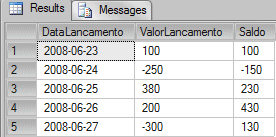
In the query above we join the table with the aggregation to return the total. Another easier, quicker and more elegant alternative would be:
|
1 2 3 4 |
SELECT DataLancamento, ValorLancamento, SUM(ValorLancamento) OVER(ORDER BY DataLancamento) AS Saldo FROM tblLancamentos AS QE |
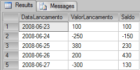
In the query above I’m using the clause OVER() with an ORDER BY. Unfortunately this will only possible with next version of SQL Server, SQL Server 2012.
Conclusion
In the next article I’ll show in more details the limitations of the window functions on SQL Server 2008 R2, and compare the performance of a running aggregation on SQL Server 2012 (Denali).
In the final and third article I’ll show in details how the window frame works. Also I’ll show how the windowing functions LEAD, LAG, FIRST_VALUE, LAST_VALUE, PERCENT_RANK and CUME_DIST works in SQL Server.
That’s all folks, see you soon with the second part of this article.
This document contains proprietary information and is protected by copyright law.
Copyright © 2026 Red Gate Software Limited. All rights reserved


Load comments