The series so far:

1. Creating Calculated Columns Using DAX
2. Creating Measures Using DAX
3. Using the DAX Calculate and Values Functions
4. Using the FILTER Function in DAX
5. Cracking DAX – the EARLIER and RANKX Functions
6. Using Calendars and Dates in Power BI
7. Creating Time-Intelligence Functions in DAX

The FILTER function works quite differently than the CALCULATE function explained in the previous article. It returns a table of the filtered rows, and sometimes it is the better approach to take.

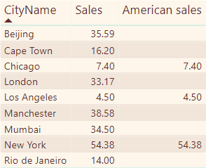
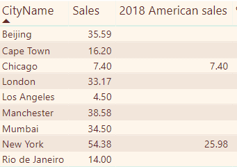
I’ll spend most of this article explaining how to create the following measures:

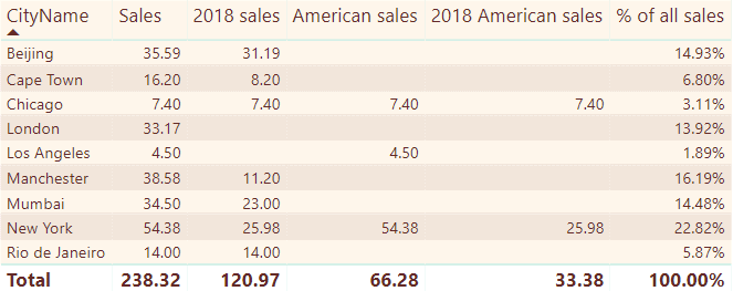
The columns above show, respectively:

1. The city name;
2. Total sales for the city in question (the filter context);
3. Total sales for the city in question for 2018;
4. Total sales for the city in question for the USA;
5. Total sales for the city in question for the USA for 2018; and
6. The percentage each city’s sales contributes to the total.

First, I’ll show you how to set up the example. Then I’ll dive into the syntax of the FILTER function. I’ll finish by highlighting the differences between the FILTER and CALCULATE functions.

A Quick Refresher

To work through the examples in this article, you’ll need to create a simple Power BI report containing a single table and then create and show a series of measures. Here’s a quick run-through of how to get started.

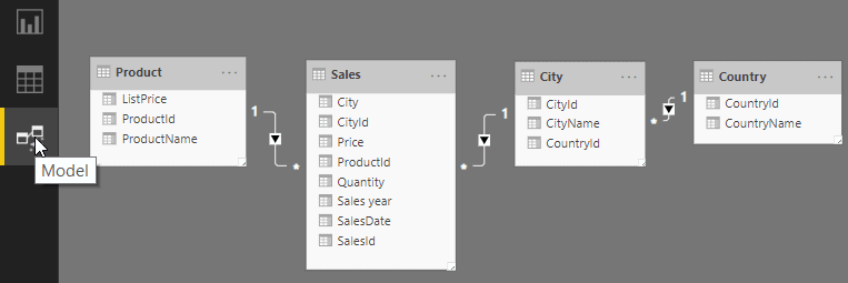
First, create a Power BI report based on the tables used in the previous articles. You can load them either from the SQL Server database given or the Excel workbook. You should now have something like this (if your diagram looks a bit different, you may not have updated your instance of Power BI to include the March 2019 update, which included the new Model View):

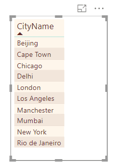
Now create a table in Report view to list out the city names. Make sure the Table visualization is selected and click CityName in the Fields list.

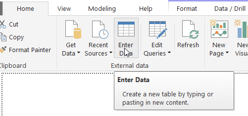
Switch to the Home ribbon and select Enter Data. This will add a new table to your report to contain your measures. To understand why you might want to do this, see this previous article in this series:

Give this table a name. Here I’ve called mine All measures:

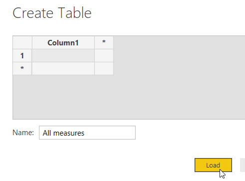
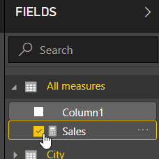
Click Load. Now add the following measure to your All measures table. You can right-click on the table and choose New measure to do this:

Choose to display this measure in your table:

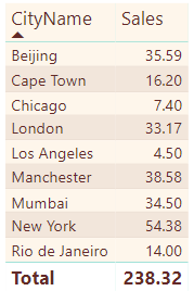
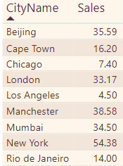
You should now be able to see the total value of sales for each city:

What happens if you want to show the sales for American cities only? Or sales taking place in 2018 only?

The FILTER Function

The measure for the sales column shown above, giving total sales for each city, is as follows:

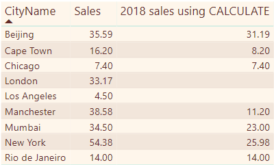
What this does (as readers of this series of articles will know) is to iterate down the rows in the Sales table, calculating the price multiplied by the quantity for each and summing the result for each city to get this:

To get the sales in 2008, you could use a CALCULATE function so that this measure would work:

This takes the filter context for each city, and further reduces it to consider only those rows where the sales occurred in 2018 to get this:

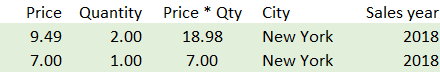
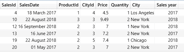
Another way to solve the problem, however, is to treat the sales for the current filter context as a table and filter it accordingly. Consider the example of sales for New York. Here’s the underlying data for this city:

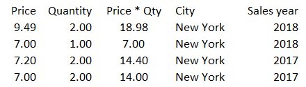
The total figure for sales for New York for 2018 is 25.98 (18.98 + 7.00). One way to get to this would be to follow these steps when compiling the data for New York. Firstly, get the data for the filter context:

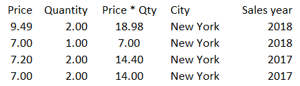
Secondly, filter this data to include only those sales for 2018, by iterating down each row deciding whether to include it. This will include only the shaded area below:

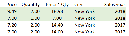
This leaves this table, which is the one whose sales Power BI will sum:

Here’s the formula to accomplish this:

This will give exactly the same results as the formula using CALCULATE above. The CALCULATE function will run more quickly because it doesn’t have to iterate down each row in the table testing a condition. At this point, you may be asking yourself what the point of the FILTER function is. I’ll return to this later in this article.

Linking tables within the Filter Function

Take a look at how to show total sales for the USA for each city. The Sales, City and Country tables are related as follows:

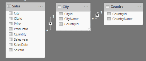
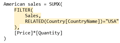
What’s needed is to iterate down the rows in the sales table, calculating the sales (price times quantity) for each but only where the country name is USA. Here’s the formula to do this:

The expression gives these results:

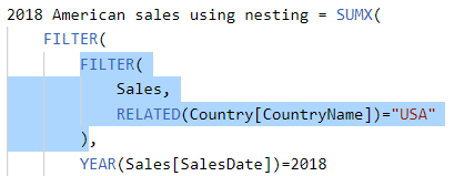
The question is – why use the RELATED function when the DAX formulae using filter context automatically link tables together? The answer is that within this formula, row context, not filter context, is used. The shaded lines in the formula below iterate over each row in the Sales table returned for the filter context, creating a row context for each:

Because within the shaded bit of the formula DAX has to create a row context for each row in the sales table, it then has to use the RELATED function to bring in the country name from the Country table.

Combining Filters Without Nesting

It’s now time to look at how to combine criteria: how to show sales which happened in 2018 and which took place in the USA. I’ll show in a bit how to do this by nesting one FILTER function within another, but for now, I’ll show ways to combine criteria. There are two basic ways to do this in DAX – either by using && or the AND function (or if either of two conditions can be true, using || or the OR function).

Here’s a version of the measure using the AND function:

Here’s the same measure, but using the && symbols:

Personally, I’d use the AND (or OR) functions any time, as they work in the same way as their Excel counterparts, and it’s easier to indent and comment formulae. However, you should use whichever floats your particular boat.

Even more sales have dropped from the figures:

Combining Conditions by Nesting Functions

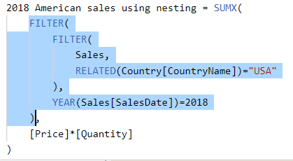
The other way to solve this would have been to nest one function within another:

Consider what this does for the New York row in the table:

Filter context restricts the data to sales for the current city in question.

The inner FILTER function iterates over each row in the table of data for the filter context, picking out only rows where the country is in the USA.

The outer FILTER function then iterates over each row in the table of sales for the USA for the filter context and applies a further constraint that the sales year must be 2018.

Depending on your data, nesting FILTER functions could speed up processing. If the vast majority of sales were outside the USA, the inner condition could eliminate nearly all rows for each city in the filter context, with the result that Power BI would only need to test the sales date for the few remaining rows.

Using ALL to Remove Any Filters

Every example shown so far has taken the set of rows for the current filter context and applied additional constraints to pick out only certain rows. However, you can use the ALL function when filtering to work with the entire table, rather than just the data for the current filter context. You could use this, for example, to show the percentage contribution of each city’s sales to the grand total:

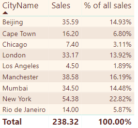
Here’s the formula for the above measure:

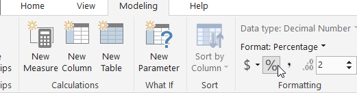
Incidentally, if you’re wondering how to get the nice percentage format, just select the measure you’ve created:

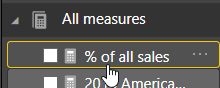
You can then set the formatting in the Modeling tab on the menu:

The Difference Between CALCULATE and FILTER

To see the difference between the way in which CALCULATE and FILTER filter data, consider this example:

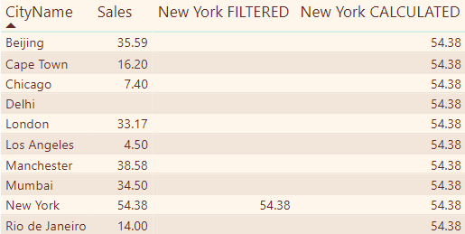
The first measure applies the filter context (so it only calculates sales for the city in question), and applies an additional constraint that the city should be New York:

The second measure replaces the filter context with a new constraint that the city should be New York, which results in the same figure appearing in every row:

Debugging Using the FILTER Function (Method 1)

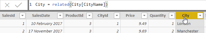
To make debugging easier, first add a couple of calculated columns to the Sales table, to give the city name and sales year. The formulae are shown below:

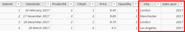
Here’s the formula for the City column. It just looks up the name of each city in which sales took place:

Here’s the formula for the Sales year column. It gives the year in which each sale took place:

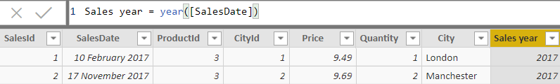
These two columns will make it easier to check what’s going on when debugging.

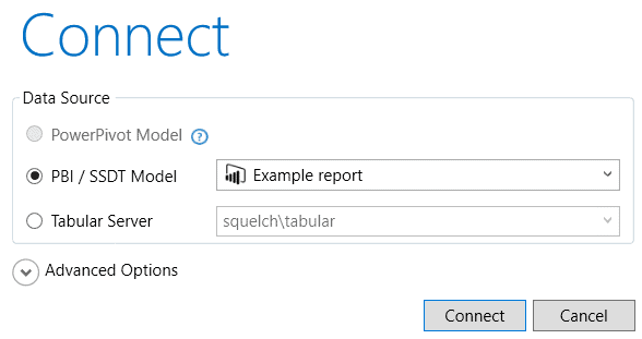
The FILTER function creates virtual tables which, under normal circumstances, you never see, but you can use a tool like DAX Studio to show the rows these virtual tables contain. I’ve covered how to download and use DAX Studio in a previous article in this series, but here’s a quick refresher. When you run DAX Studio, choose to connect to an open Power BI report:

Type in a DAX query in the top right-hand window and press the F5 key to run this. The results will appear beneath it. For the example below, I’m just listing out the contents of the Sales table:

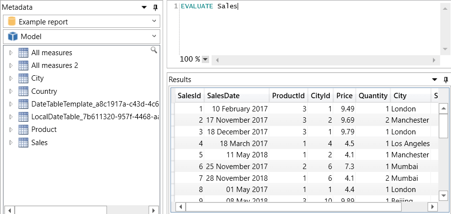
Incidentally, if you’re wondering what those long date table names are, you’re not the only one. I presume they are created behind the scenes to provide the built-in date hierarchy included in the March 2019 update of Power BI.

You can evaluate any table, including one which is returned from a filter function. A good thing to ask might be: which sales were in the United States? You can do this by copying this part of the measure you created earlier:

Precede this with the word EVALUATE in DAX Studio, and you’ll get this:

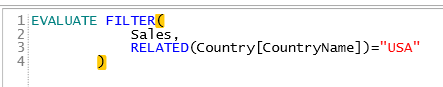
Run this to get the following output:

That’s looking good, so now you can repeat this technique with the outer bit of the FILTER function:

This gives only 3 rows:

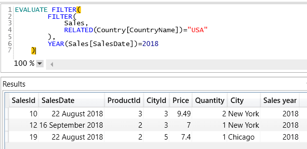
From this, it’s easy to see why you get the figures for this measure.

Debugging Using the FILTER Function (Method 2)

Another way to debug a DAX formula using the FILTER function (or any other DAX formula, for that matter) is to use variables. I’ve already covered this for scalar variables (ones holding a single value) in the previous article in this series on measures, but did you know a variable can hold an entire table?

Here’s another way to write the nested FILTER function:

The advantage of breaking the complicated formula down into different parts is that you could then test each in isolation.

Why Would You Use the FILTER Function?

I promised I would return to this question: why would you use the FILTER function when the CALCULATE function seems to offer a better alternative? There are at least four advantages:

I’ve already shown that it’s easier to debug DAX expressions that use the FILTER function.

I think expressions using the FILTER function are easier to understand than equivalent expressions just using CALCULATE.

Learning the FILTER function will help you to understand the EARLIER function, which will be the subject of the next article in this series.

There are some problems which the CALCULATE function won’t solve (an example follows).

To illustrate the last point, suppose that you want to create a measure showing total sales for cities having two or more purchases. Here are the figures that this should return:

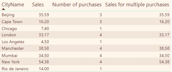
There are no sales recorded for Chicago, LA and Rio in the new measure because they each only witnessed a single sale.

Assume in all of the following that [Number of purchases] is a measure with this formula:

Here’s a measure which you could use to try to solve this problem (although it won’t work):

If you type in this measure, you’ll see the following error message:

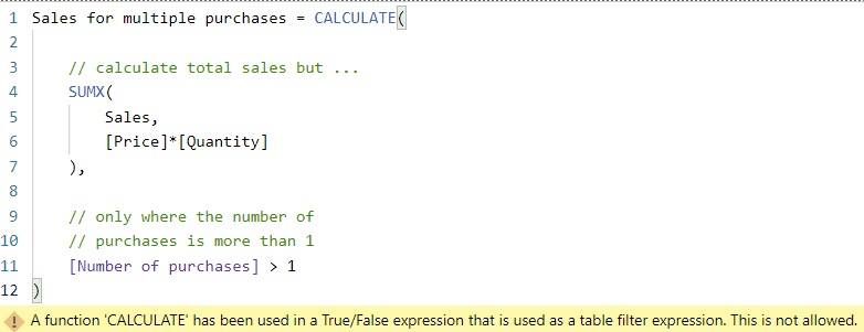
This isn’t a brilliant description of the problem, which is that you can’t use a measure in the filtering part of a CALCULATE function; you can only refer to columns. You can, however, solve this problem by rewriting it to incorporate a FILTER function:

This will calculate total sales, but only for those cities where the number of purchases was more than 1.

Summary

The FILTER function in DAX allows you to iterate down the rows of any table, creating a row context for each and testing whether the row should be included in your calculation. You can combine filters using keywords like AND and OR and also nest one filter within another. The FILTER function allows you to perform some tasks which the CALCULATE function can’t reach, and also (in my opinion) lets you create formulae which are easier to understand.