
The series so far:
- SQL Server Graph Databases - Part 1: Introduction
- SQL Server Graph Databases - Part 2: Querying Data in a Graph Database
- SQL Server Graph Databases - Part 3: Modifying Data in a Graph Database
- SQL Server Graph Databases - Part 4: Working with hierarchical data in a graph database
- SQL Server Graph Databases - Part 5: Importing Relational Data into a Graph Database
SQL Server 2017 makes it possible to implement graph databases within a relational table structure, allowing you define complex relationships between data much easier than with traditional approaches. Under this model, nodes (entities) and edges (relationships) are implemented as tables in a user-defined database, with the graph features integrated into the database engine. As a result, you can use familiar T-SQL statements to work with the graph tables, and you can use the graph features in conjunction with other SQL Server components and tools, such as columnstore indexes, Machine Learning Services, and SQL Server Management Studio (SSMS).
This article is the third in a series that covers different aspects of SQL Server graph databases. In the first two articles, you learned how to create, populate and query node and edge tables. In this article, you’ll learn how to delete and update graph data, as well as how to insert data in ways we have not yet covered.
Like the previous articles, this article includes a number of examples that target the FishGraph database, which is based on a fictitious fish-lovers forum. The database includes the FishSpecies, FishLover, and FishPost node tables and the Likes, Posts, and LinksTo edge tables. The following figure shows the data model used to build the database.
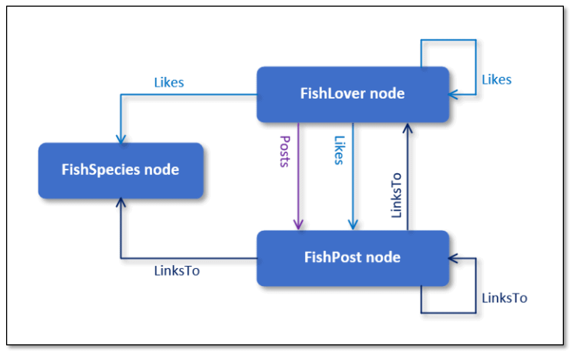
If you worked through the first two articles, this should all look familiar to you. The rectangles represent the nodes, and the arrows connecting the nodes represent the edges, with the arrows pointing in the direction of the relationships. You can download the T-SQL script used to create and populate the database at the bottom of this article.
Because we covered how to insert data in the first article, we’ll start this article with how to delete graph data and then move on to some new tricks for inserting data. We’ll leave data updates till the end because they’re not quite as straightforward as with inserting or deleting data.
Deleting Graph Data
For the most part, deleting data from a node or edge table is just like deleting data from any other table. Things only get sticky if you base your deletion on any of the auto-defined columns (node_id, $edge_id, $from_id, or $to_id), but even then, it’s not all that complicated.
Before we get into the nitty gritty of data deletion, first insert a row into the Likes table:
|
1 2 3 |
INSERT INTO Likes ($from_id, $to_id) VALUES ( (SELECT $node_id FROM FishLover WHERE FishLoverID = 2), (SELECT $node_id FROM FishPost WHERE PostID = 3)); |
The INSERT statement adds the relationship fish lover 2 likes fish post 3. You can verify that the relationship has been properly created by running the following SELECT statement:
|
1 2 3 4 5 |
SELECT Lover.Username, Post.Title FROM FishLover Lover, Likes, FishPost Post WHERE MATCH(Lover-(Likes)->Post) AND Lover.FishLoverID = 2 AND Post.PostID = 3; |
The SELECT statement uses the MATCH function to return only those rows in which a fish lover likes a fish post. The other two WHERE clause conditions refine the search to the specific user and post, giving us the following results.

I won’t go into much detail about the INSERT and SELECT statements because I covered how to add and query data in the first two articles, at least to the extent that these statements are used here. If you have any questions about what’s going on, be sure to refer back to those articles.
With that in mind, let’s look at how to delete the relationship you just added. One approach is to use subqueries in the WHERE clause to retrieve the $node_id values from the originating and terminating nodes (to try out the DELETE statements, just rerun the INSERT statement as needed):
|
1 2 3 |
DELETE Likes WHERE $from_id = (SELECT $node_id FROM FishLover WHERE FishLoverID = 2) AND $to_id = (SELECT $node_id FROM FishPost WHERE PostID = 3); |
Because the deletion is based on the values in the $from_id and $to_id columns in the Likes table, you need to compare them to $node_id values from the originating and terminating records. As you’ll recall from the first article, the database engine automatically generates the $node_id values in the node tables, creating each one as a JSON string that provides the type (node or edge), schema, table, and a BIGINT value unique to each row.
Of course, you can pass in the $node_id values as literal stings in the WHERE clause, just like you can pass in a literal string if comparing the $edge_id column (which we’ll get to shortly). However, building the JSON strings is not always as convenient as constructing subqueries. The key to using subqueries is being able to target the correct records in the originating and terminating nodes. In this case, we’re able to use the FishLoverID and PostID values from the node tables.
However, this is not the only approach you can take to deleting the data. You can also use the MATCH function to specify which relationship to delete, as shown in the following example:
|
1 2 3 4 5 |
DELETE Likes FROM FishLover Lover, Likes, FishPost Post WHERE MATCH(Lover-(Likes)->Post) AND Lover.FishLoverID = 2 AND Post.PostID = 3; |
As you’ll recall from the second article, the MATCH function lets you define a search pattern based on the relationships between nodes. You can use the function only in the WHERE clause when querying a node or edge table. In this case, the function filters out all rows except for those in which a fish lover likes a fish post. The other WHERE clause conditions ensure that that the correct relationship is deleted.
You can achieve the same results by joining the tables and foregoing the MATCH function altogether:
|
1 2 3 4 5 6 |
DELETE lk FROM Likes lk INNER JOIN FishLover fl ON lk.$from_id = fl.$node_id INNER JOIN FishPost fp ON lk.$to_id = fp.$node_id WHERE fl.FishLoverID = 2 AND fp.PostID = 3; |
All we’re doing here is joining the two node tables and one edge table. The FROM clause joins the tables based on $node_id values, and the WHERE clause filters the data based on the FishLoverID and PostID values. Although this statement is a bit more cumbersome that the preceding example, it uses a traditional T-SQL statement to delete the data, an approach that’s familiar to many.
System Functions for Graph Database
As mentioned above, you can also delete a relationship from an edge table by comparing the $edge_id column to a literal JSON value, as shown in the following example:
|
1 2 3 |
DELETE Likes WHERE $edge_id = '{"type":"edge","schema":"dbo","table":"Likes","id":15}'; |
This approach works fine as long as you don’t mind having to construct a JSON snippet every time you want to delete a row. However, SQL Server 2017 also comes with a set of built-in system functions that help simplify this process. For example, you can use the EDGE_ID_FROM_PARTS function to construct the edge ID based on the SQL Server object ID and graph ID, as shown in the following DELETE statement:
|
1 2 3 |
DECLARE @obj INT = OBJECT_ID('dbo.Likes'); DELETE Likes WHERE $edge_id = EDGE_ID_FROM_PARTS(@obj, 15); |
The object ID is the unique integer assigned to each object in a SQL Server database. The graph ID is the unique integer assigned to each $edge_id value (the id element). The id value works much like the values assigned to an IDENTITY column, with the value incremented by one with each insertion.
For this example, I used the OBJECT_ID function to retrieve the object ID for the Likes table and then assigned that value to the @obj variable, which I then passed in as the first argument when calling the EDGE_ID_FROM_PARTS function. You do not need to do this in a variable, but it can help to make the code more readable.
For the second argument, I passed in a value of 15 as the id portion of the JSON value. The key to make sure you’re passing in the correct id value. Otherwise, that’s all there is to using the EDGE_ID_FROM_PARTS function, and the other graph functions are just as basic. SQL Server 2017 includes six graph functions in all, as described in the following table.
Built-in functionDescription
|
OBJECT_ID_FROM_NODE_ID |
Extracts the object ID from a $node_id value. |
|
GRAPH_ID_FROM_NODE_ID |
Extracts the graph ID from a $node_id value. |
|
NODE_ID_FROM_PARTS |
Constructs a JSON node ID from an object ID and graph ID. |
|
OBJECT_ID_FROM_EDGE_ID |
Extracts the object ID from an $edge_id value. |
|
GRAPH_ID_FROM_EDGE_ID |
Extracts the graph ID from an $edge_id value. |
|
EDGE_ID_FROM_PARTS |
Constructs a JSON edge ID from an object ID and graph ID. |
Microsoft currently provides little information about these functions and offers no examples, but if you play around with them, you’ll quickly get a sense of how they work. No doubt we’ll eventually see more information about each function, and we might even see additional functions. Until then, the existing ones represent a good starting point, not only for deleting data, but also for building other types of queries, as you’ll see in the next section.
Revisiting Data Inserts and Data Queries
In the first article in this series, you saw several examples of how to insert data into node and edge tables. Inserting data into a node table works just like any other SQL Server table. You specify the target columns and their values and leave it to the database engine to populate the $node_id column.
If you want to remove the new row so you can try different ways to insert the same data, you can use the following DELETE statement as needed, specifying the correct FishLoverID and PostID values:
|
1 2 3 4 5 |
DELETE Likes FROM FishLover Lover, Likes, FishPost Post WHERE MATCH(Lover-(Likes)->Post) AND Lover.FishLoverID = 2 AND Post.PostID = 3; |
Edge tables are similar in this respect, except that the database provides values for the $edge_id column. However, edge tables also include the $from_id and $to_id columns, which you must manually populate when you insert data. One way to do this is to use subqueries that retrieve the $node_id values from the originating and terminating node tables, as you saw earlier in the article (duplicated here for your convenience):
|
1 2 3 |
INSERT INTO Likes ($from_id, $to_id) VALUES ( (SELECT $node_id FROM FishLover WHERE FishLoverID = 2), (SELECT $node_id FROM FishPost WHERE PostID = 3)); |
Although this approach works fine, you can instead use the NODE_ID_FROM_PARTS function to construct the $node_id values when inserting the data:
|
1 2 3 4 5 |
DECLARE @obj1 INT = OBJECT_ID('dbo.FishLover'); DECLARE @obj2 INT = OBJECT_ID('dbo.FishPost'); INSERT INTO Likes ($from_id, $to_id) VALUES ( NODE_ID_FROM_PARTS(@obj1, 1), NODE_ID_FROM_PARTS(@obj2, 2)); |
The example first obtains the object IDs from the relationship’s originating and terminating node tables and saves the IDs to the @obj1 and @obj2 variables, which are then used when calling the NODE_ID_FROM_PARTS function. (Again, you do not need to use variables.)
For the second function argument, you should use the graph IDs from the $node_id values in the originating and terminating node tables. These values are different from the FishLoverID and PostID columns because SQL Server starts at 0 when assigning the graph ID to a $node_id or $edge_id value.
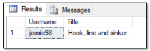
You can verify that the relationship has been correctly added to the Likes table by running the same query as earlier:
|
1 2 3 4 5 |
SELECT Lover.Username, Post.Title FROM FishLover Lover, Likes, FishPost Post WHERE MATCH(Lover-(Likes)->Post) AND Lover.FishLoverID = 2 AND Post.PostID = 3; |
If everything is working as expected, you should see the results shown in the following figure.
Up to this point in the series, the example INSERT statements left it to the database engine to generate the $node_id and $edge_id values; however, you can specify those values when inserting data. For example, the following T-SQL retrieves the object ID for the FishPost table and uses it to construct the $node_id value for the new row:
|
1 2 3 4 |
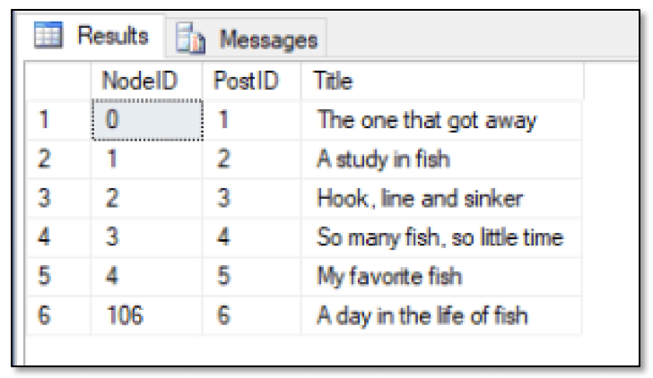
DECLARE @obj INT = OBJECT_ID('dbo.FishPost'); INSERT INTO FishPost ($node_id, Title, MessageText) VALUES (NODE_ID_FROM_PARTS(@obj, 106), 'A day in the life of fish', 'Donec pede justo, porttitor eu, consequat vitae, eleifend ac, enim.'); |
By taking this approach, you can specify what integer value to assign as the graph ID used to build the node ID (in this case, 106). This can be handy if you’re pulling data in from another source and want to use the existing ID assigned to each row as the graph ID. Just be sure to use a unique value for each graph ID, or the database engine will return an error.
Also note that SQL Server documentation briefly mentions that you cannot insert data into the $node_id or $edge_id column of a graph table. If you do, according to Microsoft, you’ll receive an error. This has not been my experience. I’ve had no problem inserting the ID values, as long as I pass them in using the correct JSON form. Because graph databases are so new to SQL Server, it’s not surprising to run into these types of inconsistencies.
With that in mind, you can verify that the row has been inserted into the FishPost statement by running the following SELECT statement:
|
1 2 |
SELECT GRAPH_ID_FROM_NODE_ID($node_id) AS NodeID, PostID, Title FROM FishPost; |
Notice that the SELECT clause uses the GRAPH_ID_FROM_NODE_ID function to return only the graph ID from each $node_id value, making it easier to confirm the value we just added. The following figure shows what the FishPost table should look like at this point.
Suppose you now want to return only the row that contains the last graph ID value inserted into the table. This can be a little tricky because SQL Server sometimes treats this type of table as though it includes two IDENTIY columns, in this case, $node_id and PostID, even though a SQL Server table can theoretically include with only one such column.
One approach you might consider to return the row is to use the @@IDENTITY system function in your WHERE clause:
|
1 2 3 4 |
SELECT GRAPH_ID_FROM_NODE_ID($node_id) AS NodeID, PostID, Title FROM FishPost WHERE GRAPH_ID_FROM_NODE_ID($node_id) = (SELECT @@IDENTITY); |
The @@IDENTITY function returns the last identity value inserted into an identity column in the current session, regardless of where the value was inserted. In this case, the function is used to compare the graph ID to the last inserted identity value. If the values match, the row is returned, as shown in the following figure.
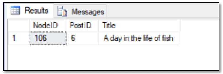
Because the SELECT statement returned the expected row, you know that the @@IDENTITY function returned a value of 106, the last inserted graph ID. (Note that you might see a different value for the PostID column if you inserted other data in the FishPost table.) You can verify that 106 is being returned by using the following statement:
|
1 |
SELECT @@IDENTITY; |
Assuming you didn’t run any other INSERT statements in your last session, you should receive the correct value.
You might also consider using the IDENT_CURRENT function rather than the @@IDENTITY function because you can target a specific table or view and it’s not limited to the current session. When calling the IDENT_CURRENT function, you must provide the name of the target table, as shown in the following example:
|
1 2 3 4 |
SELECT GRAPH_ID_FROM_NODE_ID($node_id) AS NodeID, PostID, Title FROM FishPost WHERE GRAPH_ID_FROM_NODE_ID($node_id) = (SELECT IDENT_CURRENT('FishPost')); |
Unfortunately, this approach generates no results because, in this case, the database engine returns the last value inserted into the PostID column. You can confirm this by running the following SELECT statement:
|
1 |
SELECT IDENT_CURRENT('FishPost') |
The statement returns a value of 6 rather than 106, which is why the previous SELECT statement returns no rows.
When I tried all this out, I expected the @@IDENTITY and IDENT_CURRENT functions to return the same value and could find nothing in the Microsoft fine print to suggest why they might be different. Things got even stranger when I created a node table that did not include an IDENTITY column. This time both the @@IDENTITY function and IDENT_CURRENT function returned a NULL value after I inserted a row. Next, I created a table that included the IDENTITY column but inserted a row without specifying the $node_id value. In this case, both functions returned a value of 1. In addition, my results were always the same whether or not I called the identify functions within the same batch as the INSERT statement.
Apparently, Microsoft still has some details to work out with graph databases, or I’m missing something important about how identity functions work. Just in case it’s not me, you might want to proceed with caution when using identity functions in conjunction with graph databases.
In the meantime, it you want to delete the row you just added, you can use the GRAPH_ID_FROM_NODE_ID function to extract the graph ID when comparing it to the value 106:
|
1 |
DELETE FishPost WHERE GRAPH_ID_FROM_NODE_ID($node_id) = 106; |
Clearly, the graph-related functions can come in handy at times, depending on the type of queries you’re trying to perform.
Data Updates Not Allowed
Unfortunately, the process of updating data in a graph database is not as straightforward as adding or deleting data. That’s not to say you can’t perform any updates, you just can’t perform them on the auto-defined graph columns ($node_id, $edge_id, $from_id, and $to_id).
To test this out, start with the following INSERT statement, which adds a row to the FishPost table:
|
1 2 3 4 |
DECLARE @obj INT = OBJECT_ID('dbo.FishPost'); INSERT INTO FishPost ($node_id, Title, MessageText) VALUES (NODE_ID_FROM_PARTS(@obj, 107), 'Another day, another fish', 'Donec pede justo, porttitor eu, consequat vitae, eleifend ac, enim.'); |
If you now want to modify data in one of the user-defined columns, you can run an UPDATE statement just like you would on any table. For example, the following UPDATE statement modifies the title of the row you just inserted:
|
1 2 3 |
UPDATE FishPost SET Title = 'Another data of fishing' WHERE GRAPH_ID_FROM_NODE_ID($node_id) = 107; |
If you were to query this row, you would see that the title has been updated. However, suppose you now want to update the $node_id value by changing the graph ID to 207:
|
1 2 3 |
UPDATE FishPost SET $node_id = NODE_ID_FROM_PARTS(OBJECT_ID('FishPost'), 207) WHERE GRAPH_ID_FROM_NODE_ID($node_id) = 107; |
This time, the UPDATE statement returns the following error on my system:

The same goes for trying to update the $edge_id value in an edge table:
|
1 2 3 |
UPDATE Likes SET $edge_id = EDGE_ID_FROM_PARTS(OBJECT_ID('Likes'), 216) WHERE GRAPH_ID_FROM_EDGE_ID($edge_id) = 16; |
The statement generates the same type of error as the previous statement, and the same limitation holds true for the $from_id and $to_id columns, even though these are not computed columns and you provide the values yourself. For example, the following UPDATE statement tries to update a relationship in the Likes table:
|
1 2 3 |
UPDATE Likes SET $from_id = NODE_ID_FROM_PARTS(OBJECT_ID('FishLover'), 3) WHERE GRAPH_ID_FROM_EDGE_ID($edge_id) = 16; |
Once again, you get the same error. In fact, the only way you can update an auto-defined graph column is to first delete the applicable record and then insert a new record with the correct data, as shown in the following example:
|
1 2 3 4 5 6 |
DELETE FishPost WHERE GRAPH_ID_FROM_NODE_ID($node_id) = 107; INSERT INTO FishPost ($node_id, Title, MessageText) VALUES (NODE_ID_FROM_PARTS(OBJECT_ID('dbo.FishPost'), 207), 'Another day, another fish', 'Donec pede justo, porttitor eu, consequat vitae, enim.'); |
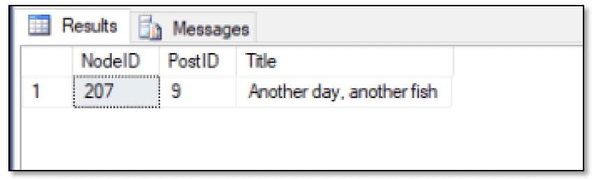
Although the graph ID value is the only data that is changing, the entire record must be deleted and a new one added. To confirm that the record has been updated, you can use the following SELECT statement:
|
1 2 3 |
SELECT GRAPH_ID_FROM_NODE_ID($node_id) AS NodeID, PostID, Title FROM FishPost WHERE GRAPH_ID_FROM_NODE_ID($node_id) = 207; |
The statement returns the results shown in the following figure, which indicates a NodeID value of 207.
As long as you know how to delete and insert records, you should have no problem performing your updates. Although this approach adds a bit of complexity to the process, it’s not too bad overall. Just be sure you delete and add the data within a single transaction.
Modifying Data in a Graph Database
For the most part, working with graph databases is fairly straightforward, once you figure out the basics of querying node and edge tables. The graph-related functions can help, but so can understanding how these tables work together to define complex relationships.
Be aware, however, that the graph database features do not include a mechanism for validating relationships. For example, you can create relationships where they don’t belong, such as a fish species liking a fish post. You can also delete a relationship’s originating or terminating record without deleting the relationships itself. For a more complete discussion of these issues, check out Dennes Torres’s excellent article SQL Graph Objects in SQL Server 2017: the Good and the Bad.
Because the tables in a graph database are similar to typical SQL Server tables, you can usually get around most limitations, as long as you understand the basics of querying and modify graph data. And the best way to learn those basics is to try the graph database features for yourself, using the type of real-world data that drives the applications you’re supporting.
This document contains proprietary information and is protected by copyright law.
Copyright © 2026 Red Gate Software Limited. All rights reserved


Load comments