

Just in case if you haven’t been following my articles, I’d better explain that I’m writing a series about the SQL Server Showplan operators. If you’re just getting started with my Showplan series, you can find a list of all my articles here.
Today, it is time to feature the Stream Aggregate operation. The operator for Stream aggregation is very common, and it is the best way to aggregate a value, because it uses data that has been previously-sorted in order to perform the aggregation quickly.
The stream aggregate is used to group some rows by one or more columns, and to calculate any aggregation expressions that are specified in the query. The commonest types of aggregation are: SUM, COUNT, AGV, MIN and MAX. When you use one of these commands, you will probably see a Stream Aggregation operator being used in the query plan. The Stream Aggregation is very fast because it requires an input that has already been ordered by the columns specified in the GROUP statement. If the aggregated data is not ordered, the Query Optimizer can firstly use a Sort operator to pre-sort the data, or it can use pre-sorted data from an index seek or a scan.
We will see later in this article how a myth is born: The Stream Aggregate is a father of this myth, but, don’t fret, we will get there in a minute, after I’ve explained how the Stream Aggregate operation works…
To illustrate the Stream Aggregate behavior, I’ll start as always by creating a table called “Pedido” (which means ‘Order’ in Portuguese). The following script will create a table and populate it with some garbage data:
|
1 2 3 4 5 6 7 8 9 10 11 12 13 14 15 16 17 18 19 20 21 22 23 24 25 26 27 28 29 30 31 32 33 |
USE tempdb GO IF OBJECT_ID('Pedido') IS NOT NULL DROP TABLE Pedido GO CREATE TABLE Pedido (ID INT IDENTITY(1,1) PRIMARY KEY, Cliente INT NOT NULL, Vendedor VARCHAR(30) NOT NULL, Quantidade SmallInt NOT NULL, Valor Numeric(18,2) NOT NULL, Data DATETIME NOT NULL) GO DECLARE @I SmallInt SET @I = 0 WHILE @I < 10 BEGIN INSERT INTO Pedido(Cliente, Vendedor, Quantidade, Valor, Data) SELECT ABS(CheckSUM(NEWID()) / 100000000), 'Fabiano', ABS(CheckSUM(NEWID()) / 10000000), ABS(CONVERT(Numeric(18,2), (CheckSUM(NEWID()) / 1000000.5))), GETDATE() - (CheckSUM(NEWID()) / 1000000) SET @I = @I + 1 END GO UPDATE Pedido SET Cliente = 1 WHERE ID IN (4,6,9) UPDATE Pedido SET Cliente = 4 WHERE ID IN (8,5,2) UPDATE Pedido SET Cliente = 20 WHERE ID IN (3,1,7,10) GO |
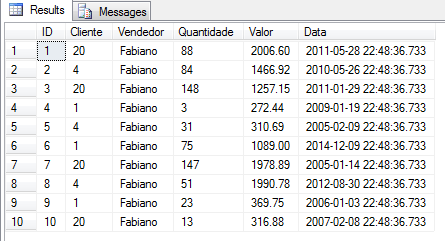
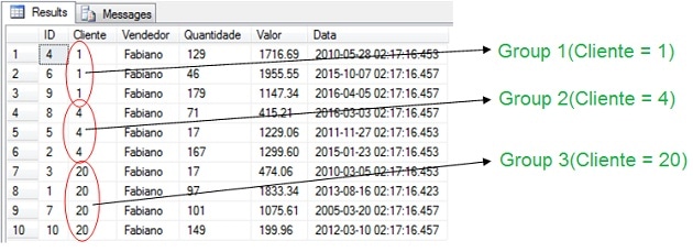
This is what the data looks like.
Let’s divide the aggregations in two types, the Scalar Aggregations and the Group Aggregations.
-
Scalar Aggregations are queries that use an aggregation function, but don’t have a GROUP BY clause, a simple sample is “SELECT COUNT(*) FROM Table”.
-
Group Aggregations are queries that have a column specified into the GROUP BY clause, for instance, “SELECT COUNT(*) FROM Table GROUP BY Col1”.
Scalar Aggregations
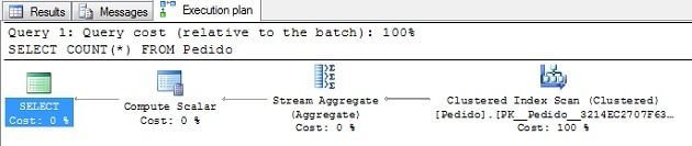
Scalar aggregations are performed using the Stream Aggregation operator. A quite simple sample is the following query that counts all rows from the Pedido table.
|
1 |
SELECT COUNT(*) FROM Pedido |
For the query above, we have the following execution plan:
Text Execution Plan:
|
1 2 3 |
|--Compute Scalar(DEFINE:([Expr1003]=CONVERT_IMPLICIT(int,[Expr1004],0))) |--Stream Aggregate(DEFINE:([Expr1004]=Count(*))) |--Clustered Index Scan(OBJECT:([tempdb].[dbo].[Pedido].[PK__Pedido__3214EC2707F6335A])) |
This is not a complicated plan. As we can see, the first step is to read the all rows from the Clustered Index. Then, as you can see this in the text execution plan, the Stream Aggregate performs the COUNT(*). After the COUNT, the result of the COUNT is placed into the Expr1004, and the Compute Scalar operator converts the Expr1004 to a Integer DataType.
You may is wondering why the Compute Scalar is needed. The answer is as follows…
The output of the Stream Aggregate is a BigInt value, and function COUNT is an Integer function. You may remember that, in order to count BigInt values, you should use the COUNT_BIG function. If you change the query above to use the COUNT_BIG, then you will see that the plan no longer uses the compute scalar operator. My great friend from SolidQ Pinal Dave gives a very good explanation about that here. There seems to be no performance advantage through using COUNT_BIG, though, since the casting operation of compute scalar takes very little CPU-effort.
Note that the Scalar Aggregations will always return at least one row, even if the table is empty.
Another important operation is when the Stream Aggregate is used to do two calculations; for instance, when you use the AVG function the Stream Aggregate actually computes the COUNT and the SUM, than divides the SUM by the COUNT in order to return the average.
We can illustrate this in practice. This query performs a simple AVG into the table Pedido.
|
1 |
SELECT AVG(Valor) FROM Pedido |
Text Execution Plan:
|
1 2 3 |
|--Compute Scalar(DEFINE:([Expr1003]=CASE WHEN [Expr1004]=(0) THEN NULL ELSE [Expr1005]/CONVERT_IMPLICIT(numeric(19,0),[Expr1004],0) END)) |--Stream Aggregate(DEFINE:([Expr1004]=Count(*), [Expr1005]=SUM([tempdb].[dbo].[Pedido].[Valor]))) |--Clustered Index Scan(OBJECT:([tempdb].[dbo].[Pedido].[PK__Pedido__3214EC2707F6335A])) |
As we can see, the Stream Aggregate calculates the COUNT and the SUM, and then the Compute Scalar divides one value by the other. You’ll notice that a CASE is used to avoid a division by zero.
Tip:
Pay very close attention that the result of the AVG will be the same type as the result of the expression contained in its argument, in our case the column specified by the query. For instance, look at the difference of the two columns of the following query.
|
1 |
SELECT AVG(Quantidade), AVG(CONVERT(Numeric(18,2),Quantidade)) FROM Pedido |
The result of the query is the following:
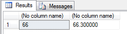
The AVG function can return int, bigint, Decimal/Numeric, money and float data, depending on the result of the expression.
Group Aggregations
Group Aggregations are queries that use the GROUP BY column. Let’s take a quite simple query to start with. The following query is aggregating all orders by each customer.
|
1 2 3 4 |
SELECT Cliente, SUM(Valor) AS Valor FROM Pedido GROUP BY Cliente |
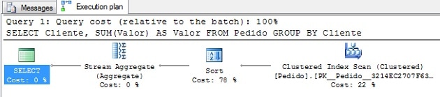
For the query above, we have the following execution plan:
Text Execution Plan:
|
1 2 3 4 |
|--Stream Aggregate(GROUP BY:([tempdb].[dbo].[Pedido].[Cliente]) DEFINE:([Expr1003]=SUM([tempdb].[dbo].[Pedido].[Valor]))) |--Sort(ORDER BY:([tempdb].[dbo].[Pedido].[Cliente] ASC)) |--Clustered Index Scan(OBJECT:([tempdb].[dbo].[Pedido].[PK__Pedido__3214EC2707F6335A])) |
The plan here is not too complicated: Firstly, SQL Server reads all the rows from the Pedido table via the Clustered Index, then sorts the rows by Customer (Cliente), with the table ordered by Customers, SQL Server then starts the aggregation: For each Customer, all rows are read, row by row, computing the value of the orders. When the Customer changes, the operator returns the actual requested row (the first Customer) and starts to aggregate this new Customer. This process is repeated until all rows are read.
The following picture shows the groups by each Customer.
As we can see from the execution plan, the sort operator costs 78% of the entire cost of the plan, which implies that, if we can avoid this step, we’ll have a considerable gain in performance.
Let’s create the properly index to see what will happens.
|
1 |
CREATE INDEX ix_Cliente ON Pedido(Cliente) INCLUDE(Valor) |
Now let’s see the execution plan.
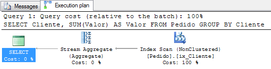
Great. It’s faster. As we can see, now the SQL Server can now take advantage of the index. It uses the ordered index by Cliente (Customer) to perform the aggregation, because the rows already are ordered by Customer, SQL doesn’t need to sort the data.
Now is time to talk about a myth about the GROUP BY clause.
a Myth is born
You probably heard from some guy that you don’t need to use the ORDER BY clause if you already put the columns into the GROUP BY. For instance, in our sample, if I write:
|
1 2 3 4 |
SELECT Cliente, SUM(Valor) AS Valor FROM Pedido GROUP BY Cliente |
… and if I want to data be returned by Cliente, you’ll be told that I don’t need to put ORDER BY Cliente clause into the query:
|
1 2 3 4 5 |
SELECT Cliente, SUM(Valor) AS Valor FROM Pedido GROUP BY Cliente ORDER BY Cliente |
Because Stream Aggregate needs to have the data ordered by the columns specified into the GROUP BY the data will generally be returned into the GROUP BY order. But this is not always true.
Since SQL Server 7.0, the Query Optimizer as two options to perform an aggregation; either by using the Stream Aggregate or a Hash Aggregate.
I’ll cover the Hash Aggregate in a next opportunity, but by now, to see the Hash Aggregate in action, we could use a very good tip from Paul Withe (you should read all his blog posts), to disable the rule used by Query Optimizer to create the execution plan using the Stream Aggregate. In other words, I’ll tell the Query Optimizer that the Stream Aggregation is not an option to create the execution plan.
|
1 2 3 4 5 6 7 8 9 10 |
DBCC TRACEON (3604); DBCC RULEOFF('GbAggToStrm'); GO SELECT Cliente, SUM(Valor) AS Valor FROM Pedido GROUP BY Cliente OPTION (RECOMPILE); GO DBCC RULEON('GbAggToStrm');â |
For the query above, we have the following execution plan:
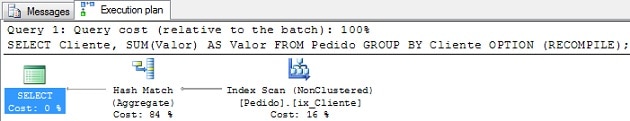
We can now see that the Query Optimizer creates a plan that uses the Hash Match (Aggregate) operator to perform the aggregation and it doesn’t require any sort operator; but that means that the rows will be returned in a random order.
So the truth is that if you need the data ordered by some column, you should, please, always put the column in the ORDER BY clause.
If the Query Optimizer chooses to use the Hash Match instead the Stream Aggregate, the data may not be returned in the expected order.
That’s all folks, I hope you’ve enjoyed this series about Operators, and I’ll hope see you next week with more “Showplan Operators”.
If you missed last week’s thrilling Showplan Operator, you can see it here.


Load comments