
If you’ve accepted Codd’s rules and you lead a purposeful life, then your concept of data is relatively simple compared to the heathens who still worship at the altar of the flat file. Your schemas are BCNF or better and your SQL isn’t polluted with RBAR; just JOINs, DRI, and a view or two.
But, there’s more to data than the RM (Relational Model). If data is your addiction of choice, I’ve got something to tempt you… statistics, embedded with relational databases. A currently prominent meme is “data science“, and the publishers are printing to a fare-thee-well. It happens that there can be an integration of the base science of mathematical statistics and relational databases to make a more integrated manifestation of “data science”. It was recently reported that R and SQL are the most-used languages of those practicing data science. In practice, that means the analyst dumps some rows from a database, imports them into a session with the statistical package, generates some output, massages this for use by a client program, puts the output in some place, rinse, repeat. “There are more things in heaven and earth, Horatio…”
My goal is to impel you to consider data science as an extension of the relational database, and even to explore the world of inferential statistics. By ‘inferential’, I mean the kind of statistics that support predictions, as opposed to descriptive statistics, which merely tell you the state of the world you’re looking at. I offer not a “how to”, but a “can do… and you can do even more”.
The way to achieve this is by using statistical packages, or ‘stat packs’. Stat packs are to the world of the mathematical statistician what DDL generators are to the professional database developer-a means for the ignorant to wreak great havoc. Having been party to ISO-9000 and Six Sigma implementations, I’ve seen the results first hand. I don’t follow their lead, anointing acolytes as statistician-lites; Instead, I encourage readers to invest some time to really understand what goes on in the field of predicting from data.
And if you’re going to do predictions from data, do it from the database… I’m not talking about vanilla stat packs talking *to* some database, for they all can do that: Rather, I’m talking about the database calling stat pack routines as it does any other engine function; different, and very intriguing .
Later in this article, I’ll be providing an example scenario using PostgreSQL (more commonly known as Postgres), since it has integration support with a stat pack. The stat pack, which has been a decade-long overnight success, is R. The name is just R. It’s an open source alternative to S, from the 1970s. Kudos to Joe Conway for writing PL/R, the R procedural language for Postgres. Note that I’m not going to advance tutorials on the constituent parts of the example (mathematical statistics, PostgreSQL, PL/R and R); there are many and the bibliography at the end of this article contains links to resources.
But before that, I’ll begin with some background information on the tools we’ll use.
Stat packs
All of the four most-known stat packs today have roots at least back to the 70s:
SAS (originally, ‘Statistical Analysis System’) is the big “kahuna” of the field. SAS is expensive, and by design, intended to be a total data management experience. Because of a decision early on to make the product a one-stop data system, it is not likely to be integrated into any particular RDBMS. SAS Institute Inc is a private company that is highly unlikely to be acquired.
SPSS (originally, ‘Statistical Package for the Social Sciences’) was bought by IBM, and is being integrated. I expect to see it being promoted for use directly in DB2 at some point. SPSS is known to be more SQL friendly than SAS.
Both SAS and SPSS emerged in the late 1960’s on mainframes (not just IBM; there really were others back then), and (along with BMDP Statistical Software), were used primarily in academic research. As an aspiring econometrician, I used them all.
Minitab is the stat pack of choice for ISO-9000 and Six Sigma contract instructors. It provides Shewhart control charts and the like. It is not what we’re looking for in our example.
There isn’t a SQL Server-centric stat pack that I’m aware of, although XLeratorDB from WestClinTech does provide some support (I’ve not used it).
So, off we go to R. R is an open source implementation of S (which is commercially offered as S-Plus), which was first developed at Bell Labs in the mid-1970s. What makes R so popular with the data analysis crowd is a very large, and growing, set of functions (available as entities called packages) written mostly in R and easily available. The main repository is CRAN. This is one case where “free” hasn’t been the impetus for adoption; it’s the large community of users/developers.
The principle difference between R and the others can be summed up, thus: SAS/SPSS/etc. are statistical command languages, while R is a statistical programming language. This difference gives R an advantage when integrating to a RDBMS.
Historically used by engineers and scientists, its host language tends strongly to Python (sorry, C#-users). R can read SQL databases with RODBC and RJDBC R-side drivers. In addition, there are R-specific database drivers, but for (mostly) open source databases: RMySql, RPostgreSQL, RSQLite, and ROracle; no RSQLServer as yet (sorry, SQL Server users). The database drivers allow more or less direct read/write of the database from R under the R-specific protocol DBI. Connecting to the database from an R client session is the usual method of integrating. In our example, we will want to run R functions against the data from the database.
There are a host of online tutorials and suchlike; some are listed in the bibliography, along with the texts I’ve used. There are a couple of other R books out, but not all that many, curiously.
Here is a review of the code base of R and the contributions: How much of R is written in R: Part 2 Contributed Packages.
Postgres and R
Postgres is, for a reason probably related to Stonebraker’s background as a coder, regarded as a programmer’s database. The Rules approach is very procedural, and differs markedly from Codd’s declarative way; not surprising in that Codd viewed the database from a mathematical and logical stance, and sought to reduce errors with a declarative structure. Folks have been arguing for decades whether declarative logic is better than procedural. Yet the coder folks are forever making frameworks and suchlike that insinuate more of the logic in declarative fashion. However, it seems they’re not yet willing to fold their tents and let the relational model win.
Postgres supports external function languages for which wrappers exist, in addition to the languages the base engine supports. This is how R can run in PostgreSQL. Since R is largely implemented in C, the wrapper runs through it. This also implies that any engine that supports C as an external language could also run R, in much the same way PostgreSQL does (hmmm…). My goal isn’t to write stat functions in R, but to call the built-ins and graph plotters.
The process of getting R and PostgreSQL up and running is a bit convoluted. The bibliography contains links to the necessary background. In one form or another R has been “embeddable” in PostgreSQL for about a decade.
For completeness: I used Ubuntu 10.04, PostgreSQL 8.4.4, R 2.13, and PL/R 8.3.0.13. The three bits of software are all available for Win and OS/X.
Stat algorithms
One last bit of background… A huge difference between the relational database world and the math stat world is that research in the latter continues to find new algorithms and implementations.
Stat algorithms tend strongly to find their expression in linear algebra, which is to say matrices, so that the data stores have historically been what relational people would possibly call first normal form tables. R has support for syntax which just about does what a relational join does; I expect that the R folks will soon enough complain about “impedance mismatch” and try to join (the verb is merge) in R. Public data, in the US anyway, is nearly always some form of flat file; some R authors even assert that such is the preferred structure. We can produce the join in PostgreSQL and pass it to the R function.
The scenario
To illustrate the possibilities when a stat/graphics pack is embedded in the RDBMS, I want a scenario where one needs to predict some future outcome based on the data. Predicting sales of nappies is boring; albeit lucrative. Let’s not do boring.
So, let’s say you’re a downtrodden political party, just having gotten smacked upside the head with a cricket bat in the last by-elections. And further, let’s say that the apparatchiks decide that some sort of data-driven application should be built to avoid the same result in the coming elections. What would such an application look like? And how would one slog through the data to find the predictive equation?
What follows is fabricated for this essay. (No politicians or political operatives were harmed in its production.) What is required here is something in between disinterested prediction (Gallop and FiveThirtyEight and so forth) and campaign strategy (“let’s go negative on my opponent and kiss supporters’ babies”): we’re not interested in simply predicting the outcome, nor will we have the authority to dictate strategy depending on what our application tells us. We want some form of feedback that can be used by the campaign decision makers, and which measures effectiveness of campaign spending, in a “Biggest Bang for The Buck” sort of way. This is the classic optimization problem from first semester calculus, but I won’t be writing derivatives.
And I don’t get to do the really cool part either: data exploration, which is the general term for spending time with a lump of data to find which general type of analysis to conduct, and having arrived at the analysis to do, working the model through the data. No, instead I’m forced to concoct a set of data which could reasonably be expected in the wild.
All logic begins with assumptions, and I’ll make some here. There is, available to the apparatchiks, both public data (the FEC here in the States) and data developed by their own organization. This latter data is, amorphously, expenditures (the source data that ends up at the FEC; their own they have, but opposition data must wait for FEC and may well not be sufficiently timely) and outcomes; perhaps simple polling results; perhaps some focus group results; perhaps some name recognition surveys. Social network data mining is also big these days (although I’ve not done enough research to know for sure that this could be a data source for outcomes). And so on. In any case, there exists reasonably objective data measuring the electability status of Our Candidates.
I’ll make the grand assumption that the organization has other data (again, some mix of public and proprietary) which can be predictive, rather than just retrospective. Such data might be: issue vulnerabilities of candidates (theirs and opposition), cultural biases among the voters, issue recognition level among voters, Q Scores.
The point here is that such data exists, but the predictive ability of any one part of the data is not known a priori. The apparatchiks have a gold mine, but they don’t know *exactly* where the gold is, and they have a relatively short time to find it. How to find the gold is the prime question. The gold may, or may not, be the simple act of spending more money on some number of candidates. This is the place to mention that studies have found that winning elections is not highly correlated with expenditures. Spending money smartly, in the Darwinist political sense, is at least as important as spending money.
Defining the objective
First, the apparatchiks must define the objective. The obvious, and naive approach is to measure $$$ spent on candidates, measure outcome (poll numbers, most likely), then send more $$$ to the candidates with the highest score, or perhaps those with the highest delta compared to previous period.
There is something wrong with that picture… The goal of our application is to identify where one will get the most bang for the buck, not where one already gets the most bang.
For example, let’s say that the organization gathers data weekly, so that it knows the $$$ and outcomes at that periodicity. Two weeks ago, John Doe was sitting at 10% of the poll, while his opponent Jack Satan was at 60%. Last week, the organization spent $1,000 on John Doe’s campaign and found that the poll numbers came out as Doe, 18% and Satan 50%. Is this sufficient information to drive a spending decision this week? The answer is “of course not”, since the logical answer must weigh John Doe’s chances against all the other ‘Our Candidates’ for the same body (say, the House of Representatives), as well as the other ‘Our Candidates’ for more significant seats (say, the Senate). Who to aid, who to abandon? Economists call this quandary “opportunity cost”; if I have the ice cream cone, I can’t also have the fish and chips (easy decision, that).
The answer to the question is “triage of the candidates”, and “data” is how one accomplishes this. For those that haven’t watched “MASH” in a while, triage is the process for dealing with mass casualties, and given the number of elections conducted in large countries, mass casualties is an apt metaphor. So, the rules of triage:
- Let those too sick to help, die.
- Let those healthy enough to live, go on without intervention.
- Help those who might live with … help.
In the case of John Doe, depending on other factors he’s a goner; sending limited money his way is wasted. By ‘other factors’, I mean such things as time left to election, or his opponent’s closet full of skeletons soon to be revealed. How, on the other hand, do we identify the non-obvious Lazarus? Can data be of any help? If so, how to do this?
Is an RDBMS the solution?
And, of course, the answer is “mostly, no”. “Mostly”, because the answer is statistical and graphical in nature, about which the relational model has not much to offer analytically; these disciplines are designed around the cursed flat file. For operational purposes, one would expect that most of the expenditure data will be in some database. It’s also safe to assume that this will be the driving data-store for the application. So, while we can expect that some of our data will be stored in a relational database, and that off-line data can be loaded with it, the relational capabilities don’t solve our problem: How to find the best candidates to support.
Once we have extracted the predictions, the second objective is to find the optimum way to display the predictions. For this illustration, I’ll say that they’ve decided on x-y plots with regression fitted. R offers an embarrassment of riches with regard to graphic display of data. You really should have a look.
In this example, I’ll ignore the client side development, which could be Ruby on Rails, Cakewalk, some .NET framework, Struts, TurboGears, and so on; the whole point is to be client code agnostic (for an real world example, visit Xtuple). Right now, all I’ll describe is using the statistics and graphing capabilities of R directly from a RDBMS, Postgres, in order to accomplish one task. I’ll assume that the client side coders will decide where and when to display the analytical results. Those results, I’ll assume for this illustration, will be some plot of our composite data, including a predictive component. The applied statistician often turns to linear regression for this situation. Econometricians and psychometricians (biostats, not so much) are long time users of regression analysis.
The implementation
We can assume, for this illustration, that we don’t have access to the apparatchiks’ proprietary data.
There is a trove of data at the FEC (Federal Election Commission), but I won’t be using the FEC data here, since I want to build a database which directly addresses the triage problem with data that the organization should have.
We proceed to winnow our data with some multivariate analysis. The essence of inferential statistics is correlation. I assume that the apparatchiks have many distinct data values available beyond what we can find in public sources. In order to demonstrate the process, I’ll make up some data names and some data. In the real world, our apparatchiks will have (hopefully) more.
Triage: The Tech Bits
First, I found this link as I wrote today, which is further evidence of my thesis: analytics/stats will be done from the database. Whether these will only be various open source databases (and, considering Oracle’s behaviour, MySql is no longer the most likely candidate) and stat packs remains to be seen. But the momentum is building. I am by no means a fan of NoSql type datastores, and for R support, it seems a bad match: That said, events move apace.
As I was preparing the TechBits, PostgreSQL v 9.1 went official. One of the new features is a K nearest neighbor indexing. Unless the Postgres folks enjoy confusing their users by munging a term they should be well aware of, K nearest neighbor is used in classification analysis, which R supports: More evidence that stats are being merged with the relational database.
For the purposes of this demonstration, I’ll assume that, whatever the underlying catalog, a simple view can be constructed for our use. I’ll also abstract away various niceties such as sql injection barriers (Postgres does it much the same as others), data normalization, and any other tasks needed to concoct an appropriate view.
Here’s the data table:
|
1 2 3 4 5 6 7 8 9 |
CREATE TABLE "public"."events" ( "period" int4 NOT NULL, "candidate" varchar(25) NOT NULL, "event" int4 NOT NULL, "amount" int4 NOT NULL, "outcome" int4 NOT NULL, "choice" int4 NOT NULL, "guncontrol" int4 NOT NULL ); |
The categorical columns, choice, guncontrol, are common 5 point scale from “Strongly Disagree” to “Strongly Agree”, and reflect the candidate’s position, not the voters (in this data, John Doe displays fungible positions). Adding the voters’ view is certainly useful. I’ll also assume that these are the minimal wedge issues, though more can be expected; which leads to the matter of data for stats. Stat calculations just don’t work on character data, so it must be translated. Here, they have already been. The same translation is required for event, so I’ll define the value/string such:
- debate
- canvas
- rally
- radio advert
- TV advert
The ordering is approximately monotonic in cost to execute; the apparatchiks would order them that way, in any event.
The naive’ notion is that measuring outcome, which in this data is the normalized polling percent, e.g. 11 is .11 or 11%, after spending money is sufficient information to shape further expenditures. The organization will have data for all candidates across the country; the question is who gets how much this week or month or quarter. Visual display of two variables is simple: a scatterplot with a simple regression line through the points. And, since in this notion, the data are nicely continuous, it makes sense in the arithmetic.
In Postgres, all “code” is stored as functions (functions, stored procedures, and triggers). Here’s the function to generate a scatterplot and regression lines for our data.
|
1 2 3 4 5 6 7 8 9 10 |
CREATE OR REPLACE FUNCTION "public"."pairs_graph" () RETURNS text AS $BODY$ X11(display=':5'); events <- pg.spi.exec ("select period, event, amount, choice, guncontrol, outcome from public.events where candidate = 'Doe' "); pdf('pairs_graph.pdf'); pairs(events,panel=panel.smooth); dev.off(); print('done'); $BODY$ LANGUAGE 'plr' |
- The $BODY$ lines are markers to the engine for code blocks.
- The X11 line is required by Ubuntu to write graphs to files; the reasons are covered in the Ubuntu link.
- The events line does the database work; the <- is assignment to a dataframe, what we want as the explained variable, outcome, is listed last for visual ease.
- The pdf line tells R/Postgres where to write the graph; this will be in Postgres’ home path.
- The pairs line does the work; it generates pairwise scatterplots and fitted regressions (many options are available).
- The dev.off line disconnects from X11
- Finally, print sends a soothing message to the console.
Note that language is called as ‘plr’; it’s actually C, since R (entry points, in any case) is a C application.
We live in a three dimensional world, cosmologists not withstanding, and even displaying three axes of data leaves most people puzzled. We want to predict outcomes driven by more than one predictor, money. We want to do it graphically, but we really only have two dimensions to work with. It turns out that R provides support for that. Traditionally, multiple regression would print text, not graphs.
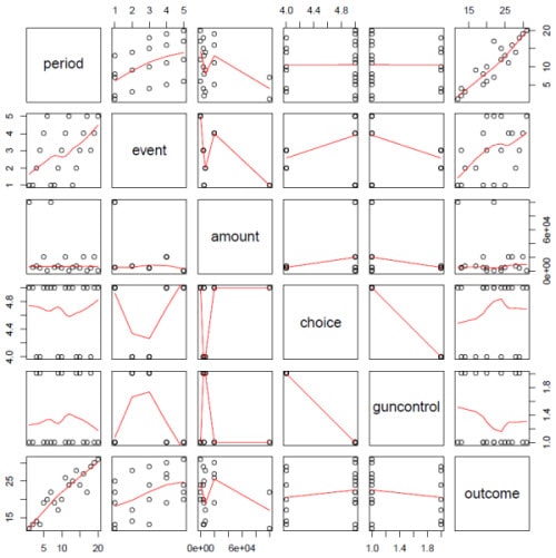
What does this tell us? The row we care most about is the last, where outcome is plotted against each of the explanatory variables. Time is a great healer in this data. Amount spent, not so much. Most significantly, R fits what are called localized regression lines which adapt the slope of the fit for changes in the scatter; this is why the lines aren’t just straight, as one would get from a simple regression. The advantage of this method is better fit, at the cost of complexity. Localized regression is a stat algorithm, not specific to R.
Interpretation during such a PoC/prototyping/agile exercise raises meaningful questions for our apparatchiks. Here are just a few.
Do we find, looking at the other rows in the panel, that our presumed independent variables are correlated? The real world implication, if there is correlation, is that overall predictability of our variables isn’t quite as good as the calculations show (we don’t print them for this GUI widget). It also could mean that these factors’ correlation was unknown to us. We’ve learned something about our data; some variables affect others in ways we didn’t understand. For example, gun control and choice are negatively correlated. That’s likely true with real data, too. Depending on the attributes tracked, correlations among the explanatory variables offers the opportunity to hone our funding process. There may be insurmountable effects in the electorate such as gun control and choice. There may be opportunities; immigration may be less significant than hypothesized.
Do we measure outcome with just one source? Sources can include our pollster who may gild the lily a bit to keep the Suits happy, Gallup, or similar, polling, name recognition surveys, social network mining (what happens on twits/tweets and facebooks, etc. after an event), radio/TV ratings, opposition response. We can define a composite outcome, weighting each component as the apparatchiks see fit.
How do we measure outcome, point in time or delta? We can see the trend on the period graph in the panel using point in time. We could also plot delta-outcome against the variables. It may well be that $10,000 will be enough to move from 10% to 11% (a 10% gain), but a 10% gain on a base approval of 40% (delta-outcome 4 points) may never happen; the curve bends down.
What is the weight of John Doe in the organization’s nationwide plan of attack? Does Doe matter more or less than Smith in another district? Is Doe a shoe-in? All of these matters impinge on the funding decision which the stats are intended to guide; who among the wounded are most likely to prevail with assistance? Who is gaining traction, and who is slip sliding away? We can now query our database, and provide a semblance of an answer to our suits in a pretty GUI.
Since we can graph for an individual, do we also provide graphs on aggregates; for example, all candidates for all seats in a state, or by region (here in the States, Red versus Blue is popular)? We can aggregate up in either sql or R. A reasonable UI would be a map of the country. A right click on a state/province/canton would bring up a list of candidates by district, the user picks the candidate then chooses the factor attributes to plot (in addition to outcome, event, and amount), and choosing would return the panel for that candidate. A rollup at the state/etc. level would need weights for each candidate, assigned by our apparatchiks; upper chamber being more important, influential districts, and the like.
This panel display, with half a dozen variables, is about the limit for a naive’ (from the point of view of stat sophistication) user. With exposure, and perhaps some instruction, sophistication develops rather quickly and the response is always for more data. At one time, I taught one week stat courses for the US government. We didn’t have R, but the kernel of stat thinking gets through. That kernel: from a computational standpoint, it’s all about minimizing squared differences. We tell R to find the best model to fit the data we have (and *not* the other way round), by minimizing the differences between the data points and the model’s graph. There’s a whole lot of maths behind that, but you only need to know them if you’re determined to acquire a degree in stats. Or write R routines! What applied stats (by whatever title) folks need to keep in mind are the assumptions underlying the arithmetic their stat pack is implementing. Most often, the assumption that matters is normality in the data. The stats meaning of “normal” is similar to what RDBMS folks mean. Both fields have orthogonality as a principle: for RDBMS, “one fact, one place, one time”; for stats, all independent variables are also independent of themselves. The larger meaning for stats folks is that the variables follow a normal/bell curve/Gaussian distribution. This assumption should be confirmed. Stat packs, R included, provide tests for this and should be exercised and methods for transforming variables such that they are more nearly normal in distribution.
But for our apparatchiks, there’s plenty of exploration to be had. That would be done in the usual fashion: connecting to a relational database from R in R Studio. From that vantage, correlations in the data, hints of what other data might be useful, what sorts of visual displays, and much more can be discovered. At that point, creating functions in Postgres to present the visuals is a small matter, the script in R Studio can (nearly) be dropped into the Postgres function skeleton, just add the SQL query.
As above, the client side code will have some glyph to click, which represents a candidate. Clicking the glyph will bring up the plot. For a web application, we need only have the image file on the web server’s path. We’ll supply some form of a graphics file such as png or pdf. For my purposes, providing a point plot in an OS file will suffice. In fact, since all industrial strength databases support BLOBs/CLOBs, we could store images in the database, and serve them up (I’ll leave that as an exercise for the reader). (For what it’s worth, my research showed that discussions come down on the side of OS files rather than BLOBs.) For a web application, writing to an OS file is fine; we only need to fill in the img tag to get our plot.
In order to run R functions, we need some help. That help is in the form of PL/R, the driver that “embeds” the R interpreter in Postgres. Once PL/R has been installed, we can use R functions in our SELECT statements. We can then run R functions in Postgres that produce text output, and, more to the point, graph image files. These can then be shipped off to the client code. Kinda cool.
So what does the future hold?
For some time, ANSI SQL has been accruing ever more complex statistical functions; there’s even support for regression, although I must admit, I’ve never quite understood why-anyone experienced enough to understand what regression does wouldn’t trust a RDBMS engine (well, its coders, really) to do it justice.
When IBM bought up SPSS Inc, it sent a shiver down my spine. A good shiver, actually, since I’d been born into professional employment as an econometrician, and used SPSS in its early mainframe clothes. I expect DB2 to include SPSS commands, thus thumbing their nose at ANSI. But, with other developments in the hardware world (multi-core/processor and SSD) why not? What with some ANSI sanctioned stat calculations, the BI world nudging up against the OLTP world (near real-time updating), and the advent of (possibly) full SSD storage for RDBMS, what might the near future look like?
Now that IBM has SPSS, and Oracle has bulked up on some stats (but I don’t find a record of them buying up a stat pack vendor, and what they show is nowhere near R), might SQL Server integrate to R? Or, Oracle? It’d be easier for Oracle, since the engine already supports external C functions. SQL Server is mostly(?) C, so adding C as an external function language shouldn’t be a mountain to climb.
R is GPL, and calling GPL software doesn’t make the caller GPL; that’s been established for years. If it were otherwise, no-one would run Apache or most versions of WebSphere. Calling into R from the engine is no different. The PL/R integration was written by one person, Joe Conway, and given that both Oracle and Microsoft have legions of coders at their disposal it wouldn’t be much more than a molehill for them to write their own integration. And if the Oracle or Microsoft coders chose to write a new solver for R, that code would also be under GPL.
My hope, and I’ll qualify that as a ‘guess’, is that “fast join databases” will become the norm (since they’ll be highly normal), which, along with federation, removes the need for separate DW databases being fed from OLTP databases. There’ll just be one database, just like Dr. Codd envisioned, supporting all applications in need of the data. And, yes, decent federation support deals with disparate data types across engines. With stat pack syntax built into SQL (SSQL, perhaps?), the database server becomes a one-stop shopping center. Just don’t expect an ANSI anointed standard.
Bibliography and links
I’ve ordered the bibliography “from soup to nuts”, rather than the traditional alpha sort. The texts are those I have used, and a few with high regard in the community that I’ve not gotten to yet.
- Postgres installation.
- Matthew and Stones: “Beginning Databases with PostgreSQL”. Almost everything needed to get running with Postgres.
- An R installation instruction.
- R for Windows: FAQ.
- R Studio. An open source, all platform, IDE entrance to R. Quite new. To quote the end of Raiders of the Lost Ark, “It’s beautiful”. No, your head won’t melt.
- Installing PL/R. From the Onlie Beggeter of PL/R; follow the link back.
- Using PL/R. Very helpful information.
- Ruby: If you only want this for FECHell, follow the links to 1.8.7; 1.9.x and FECHell don’t get along. Otherwise, use rvm or similar to have multiple Rubys on your machine.
- Python. Take 2.7.x; Python is the lingua franca of the R/stats world. Optional to this article.
- FECHell. If you want to explore US election spending…
- Adler: “R in a Nutshell”. The most comprehensive, although necessarily not deep, coverage; if you’ve got a question, you’re most likely to find the answer here.
- Maindonald and Braun: “Data Analysis and Graphics Using R”. I have the second edition, from 2007; from the comments, there’s not much difference. Stresses the graphics, and the R code is relegated to footnotes!
- Crawley: “The R Book”. The best all rounder.
- Chambers: “Software for Data Analysis”. Written from a programmer’s, rather than analyst’s or user’s, perspective.
- Wickham: “ggplot2 Elegant Graphics for Data Analysis”. The latest plotting function, in depth. The graphs and plots here weren’t made with ggplot2, I’ve not dug into it enough.
- Venables and Ripley: “Modern Applied Statistics with S”. The lodestone text; syntax is S, and from 2002 or thereabouts.
- Cleveland: “The Elements of Graphing Data”. Cited, where any book is, as the graphics source in R; if you were expecting Tufte (I was), sorry.
- Hoel: “Introduction to Mathematical Statistics” My stat book.
- Janert: “Data Analysis with Open Source Tools” A practitioner’s take on data analysis, not mostly R and not mostly regression; likely an older guy, with much snark on offer, and much of it earned.
- Ubuntu specific gnarls: Some needed tidbits dealing with plot production.
This is my fave online tutorial, although I’ve not got the book derived from the tutorial.
And, for all things R online, there’s R-bloggers.
Glossary
- BI: Business Intelligence
- BNCF: Boyce-Codd Normal Form
- BLOB: Binary Large OBject
- CLOB: Character Large OBject
- DBI: Database Interface
- DDL: Data Definition Language
- DRI: Declarative Referential Integrity
- DW: Data Warehouse
- FEC: Federal Election Commission
- GPL: General Public License
- OLTP: OnLine Transaction Processing
- OS: Operating System
- PL/R: Procedural Language for R
- RBAR: Row by Agonizing Row
- RDBMS: Relational Database Management System
- RJDBC: a package implementing DBI in R on the basis of JDBC (Java Database Connectivity)
- RM: Relational Model
- RODBC: a package implementing DBI in R on the basis of ODBC (Open Database Connectivity)
- SAS: Statistical Analysis System
- SPSS: Statistical Package for the Social Sciences
- SSD: Solid State Drive
This document contains proprietary information and is protected by copyright law.
Copyright © 2026 Red Gate Software Limited. All rights reserved
Load comments