Over the years, SQL Server Statistics have been discussed in countless blog posts, articles, and presentations, and I believe that they will remain a core topic for a while when speaking about performance. Why is that? Well, if we were to consider the equivalent of Maslow’s hierarchy of needs for database performances, statistics would be a foundational needs of a database system (namely the “physiological” needs) as they are one of the most fundamental pieces of information needed to build execution plans.

That being said, accurate statistics are not likely to help in all situations: you can think of poorly written queries, table-valued parameters (TVP), incorrect model assumptions in the cardinality estimator (CE), parameter sensitive plans (PSP) and so on. But I believe that it is worth it to check if they are “accurate enough” to avoid having a blind spot in this area.

In this article, we assume that the reader is familiar with the basics of SQL Server statistics, so we will focus on a question that seems simple at first glance: are statistics “accurate enough”? Should you need more information before diving in this article, feel free to have a look at these great articles: the basics and problems and solutions.

If you have already searched a bit on this topic, it is possible that the answer you have most often found to this question can be summarized by “it depends” combined with “test on your systems”. Not bad advice, but some people have pushed it a bit further, and one of the best approaches that I would recommend has been published by Kimberley L. Tripp. It put me on track a couple of months ago, and I have been lucky enough to be allowed to work on this topic as part of my current role as performance engineer.

We will start by trying to understand what “accurate enough” means, what are the main factors affecting statistics accuracy, then we will explain and demonstrate a process to analyze and try to tune statistics. In the last section we will see how you could give it a try, what to do when the sampling rate cannot be increased or when it will not increase statistics accuracy, and finally how modern versions of SQL Server may help to tackle this problem.

What is “accurate enough”?

KIS (keep it simple!) To keep it simple, we can consider that statistics are accurate enough when they are not the root cause of significant discrepancies between the estimates and the actuals leading to the creation (and possibly caching) of poorly performing execution plans, which may also consume much more resources than required. With “accurate enough” statistics, we increase our chances of building execution plans for realistic data volumes, so the plan trees chosen (e.g. sequence, operators) and the resources granted (e.g. memory) are more likely to deliver optimal performances.

Accuracy importance is relative

It is important to keep in mind that a workload that is likely to seek or scan very large ranges of data is typically less sensitive to inaccurate statistics: the larger the range, the more “smoothed out” the inaccuracies. On the other hand, a workload that is looking for discrete data points is more likely to be sensitive to inaccurate statistics. Also, as mentioned in the introduction, there are a number of situations where the accuracy of the statistics may not matter much:

• when the query is so simple that it gets a trivial plan
• when using a table-valued parameter (TVP) – which do not have statistics, at the very best we have a cardinality estimates (estimated number of rows)
• when using local variables or the query hint OPTIMIZE_FOR_UNKNOWN
• when incorrect model assumptions are used by the cardinality estimator (CE)

So yes, despite your efforts to build accurate statistics, you may end up with estimates based on the density vector or fixed guesses – and the outcome will not necessarily be bad! And when parameter sensitive plans (PSP) arise, you may get the perfect plan for the parameters used at compile time, but unfortunately these parameters may not be representative of most of the calls so the plan built for them may perform poorly for most of the calls.

Factors affecting statistics accuracy

In this section I will look at a few of the things that can affect how accurate statistics are for any given table.

Write activity

We can use the columns “last_updated” and “modification_counter” exposed by the Dynamic Management Function (DMF) sys.dm_db_statistics_properties to identify the date and time the statistics object was last updated and the total number of modifications for the leading statistics column (the column on which the histogram is built) since the last time statistics were updated. We can also rely on a mix of technical knowledge, business knowledge and experience to identify when an update of statistics could be worth it (e.g. after an ETL load, at the end of the year-end closing…), in addition to automatic and/or scheduled updates.

However, as tempting as it may appear, updating statistics often to keep them synchronized with the updates performed on the database should be considered with caution because:

• it has a cost (CPU, IOs, tempdb)
• it may degrade the statistics accuracy (e.g. when using the default sampling rate whereas the last update has been performed during an index rebuild – meaning with full scan)
• it may invalidate cached execution plans, and it might be difficult to predict if the new plan will be as “good” as the previous one
• by default, automatic updates of statistics are synchronous so the query optimizer will wait for the statistics to be (re)computed to (re)compile the execution plan, hence delaying query execution (can be asynchronous but to use with caution)
• the default CE does a better job at estimating the number of rows beyond the histogram than the legacy CE, the legacy CE could leverage the trace flags 2389 / 2390 to help in some situations (and both CE could leverage 4139!)

So, having the automatic updates of statistics enabled plus a scheduled update process (e.g. weekly) is generally a good practice, but it is definitely not a “one-size-fits-all”. And finally, should you want to dive deeper into the impact of this factor which will not be covered in this article, you can have a look at this excellent article from Erin Stellato.

Sampling rate

From the DMF sys.dm_db_statistics_properties mentioned above, an important bit of information is exposed in the “rows_sampled” column. This is the total number of rows sampled for statistics calculations. By default, this number is primarily based on the table size, as explained in this MS blog archive SQL Server Statistics: Explained and demonstrated by Joe Sack in Auto-Update Stats Default Sampling Test. So, by default, the sampling rate (rows_sampled/rows*100) ranges from 100% (full scan) for tables smaller than 8MB to less than 1% for large tables.

The algorithm defining the number of rows to sample has been designed so on most of the systems StatMan (internal program in charge of computing statistics) should produce the best statistics possible with as few resources as possible (CPU, IOs, tempdb) and as fast as possible. As you can guess, it is a very challenging task but it does a great job as this works quite well for the vast majority of statistics.

Data pattern

Then, the sampling rate alone does not dictate the accuracy of the statistics. A low sampling rate may be perfectly acceptable for data that can have only few distinct values (e.g. status code, active status, etc) or data that are evenly distributed (e.g. a column with an identity property) but it is likely to generate inaccurate statistics for data that can have a lot of values (e.g. thousands of customers) or unevenly distributed data (e.g. if the sales activity has huge variations). The challenge of getting accurate estimates for specific data points could be summarized as below:

So, when focusing on specific data points, even if statistics are updated with full scan the estimates may be completely wrong. To be more specific, if there are no updates on the underlying data the details of the statistics (density vectors and histogram steps properties) will be perfectly accurate, but it may not be enough. As we are limited to 201 steps (200 for actual values, plus 1 for nulls) in the histograms, the dispersion around the mean (the “average_range_rows”) may be extremely important. Said differently, the actual number of rows matching a specific value in the range of such steps may vary widely.

Analyze and Tune Statistics

Now that we have introduced the core factors affecting statistics accuracy, we will see how we could automatically evaluate the accuracy of statistics (analysis phase) and if we can improve the accuracy of statistics – when it is worth it and possible – by using a custom sampling rate (tuning phase). A stored procedure named sp_AnalyzeAndTuneStatistics will implement the analysis and tuning logic. In this section, we will outline how it works, its input parameters and perform a demo.

Note that the algorithm will skip graph tables as there are some differences in the internals that make it beyond the scope of this article.

The code for this stored procedure can be downloaded in .zip format here from the Simple-Talk site.

How it works

Let’s start with the analysis phase. From a high-level point of view, this phase gets the statistics eligible for an analysis in the current database and loops on each of them to:

• Update the statistic (using the default sampling rate)
• Based on the representation in the histogram (found using DBCC SHOW_STATISTICS), analyze the base table to compute actual equal_rows, actual average_range_rows and coefficient of variation in the range (dispersion around average_range_rows)
• Count the number of steps having a difference factor above the maximum difference factor passed as input parameter (by comparing estimated and actual equal_rows and average_range_rows) and the number of steps having a coefficient of variation above the maximum coefficient of variation passed as input parameter
• Log the results

So, at the end of the analysis phase, we can review the logs to find out for each statistic analyzed how many steps are above the thresholds passed as input parameters. These steps will be qualified as “not compliant” (with the thresholds) from now on.

Then, when the mode “tuning” is enabled (see the statement block related to “IF @p_TryTuning=1” in the procedure), a nested loop is activated in the loop on each statistic, so after the initial analysis:

• the statistic is updated with a larger sampling rate
• a new analysis is executed
• if the new number of steps not compliant drops quickly enough, the nested loop is repeated, otherwise the tuning phase stops

The goal is basically to identify the “low hanging fruit”, meaning the statistics which accuracy may experience an improvement with a limited increase of the sampling rate. But how do we assess if the number of steps not compliant drops quickly enough? We will use the concept of slope. The steeper the slope, the faster an improvement is expected, meaning the faster the number of steps not compliant have to drop after each increase of the sampling rate. The steepness of the slope will be set by the input parameter named “slope steepness”: the higher it is, the steeper the slope (and vice-versa).

So, the formulas to compute the maximum number of steps not compliant for a given sampling rate use a parameter (prefixed with “@p_”) and a couple of variables computed during the execution (prefixed with “@v_”):

• @v_NbStepsExceedingDifferenceFactorInitial: the initial number of steps having a difference factor exceeding @p_MaxDifferenceFactor (see Input parameters below), using the default sampling rate
• @v_NbStepsExceedingCoVInitial: the initial number of steps having a coefficient of variation exceeding @p_MaxCoV (see Input parameters below), using the default sampling rate
• @p_SlopeSteepness: the slope steepness (see Input parameters below)
• @v_SamplingRateAssessed: the sampling rate assessed
• @v_DefaultSamplingRate: the default sampling rate

And are computed this way:

• For the maximum number of steps not compliant in terms of difference factor

• For the maximum number of steps not compliant in terms of coefficient of variation

Note: the significance used for the function FLOOR is 1

You can see below a representation of the maximum number of steps not compliant acceptable for @p_SlopeSteepness = 25 (default value), @v_DefaultSamplingRate = 10 and @v_NbStepsExceedingDifferenceFactorInitial = 50:

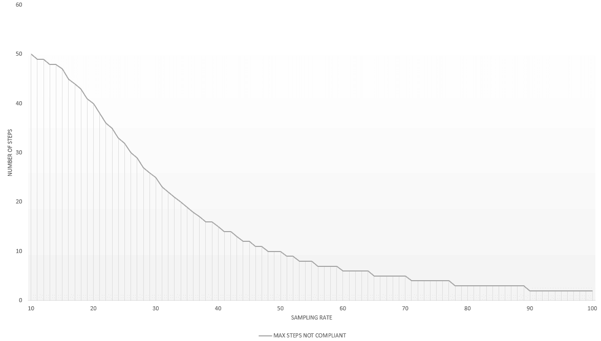
And the same representation for p_SlopeSteepness = 100:

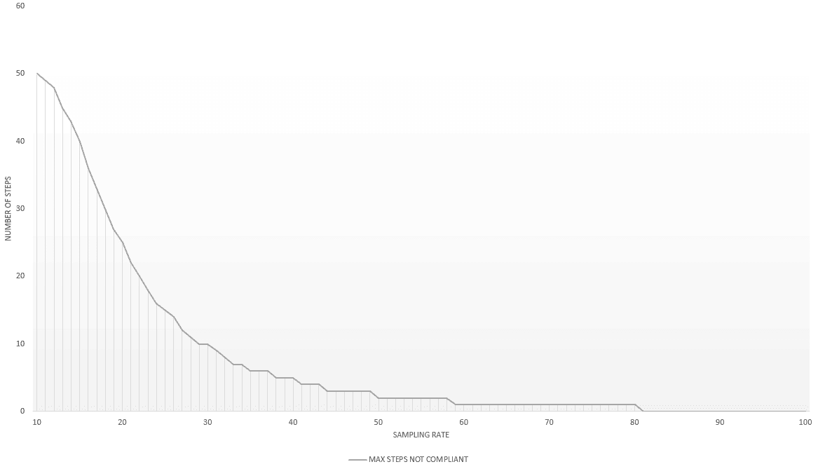
As you can see, the steeper the slope, the faster the number of steps not compliant have to drop.

Input parameters

Let’s now have a look at the input parameters of the stored procedure so it can be clearer how the process works to gather the information on statistics.

@p_MaxDifferenceFactor

Maximum factor of difference accepted between estimates and actuals, to assess equal_rows and avg_range_rows accuracy in each step of the histograms. If the factor of difference of the step for equal_rows or avg_range_rows is above the value of this parameter, the step is considered “not accurate enough” (not compliant). It is computed by dividing the largest value (estimated or actual) by the smallest value (estimated or actual), to consider underestimations and overestimations similarly.

Example 1:

the estimated number of rows equal to the range high value (equal_rows) is 100

the actual number of rows equal to the range high value (equal_rows) is 1000

=> the factor of difference for equal_rows is 10

Example 2:

the estimated average number of rows per distinct value in the range (avg_range_rows) is 1000

the actual average number of rows per distinct value in the range (avg_range_rows) is 100

=> the factor of difference for avg_range_rows is 10

This parameter has a default value of 10. It could be considered large, but this is by design as we want to focus on significant discrepancies. Of course, it is not great to have an actual number of rows that is larger or smaller by a factor of 6 or 8 but is it much more likely to cause performance issues when it is larger or smaller by a factor above 10.

@p_MaxCoV

Maximum coefficient of variation accepted in the histogram ranges, to assess the dispersion around avg_range_rows. It is expressed as a percentage and has a default value of 1000. This default value could also be considered large but this is by design as we want to focus on significant discrepancies.

@p_SchemaName, @p_ObjectName, @p_StatName

If you want to filter by the schema, object, and/or statistic name, this parameters let you. By default the value is NULL which is not applying a filter.

@p_TryTuning

To activate the tuning phase where statistics are actually updated, By default this is set to 0 and will not make changes to statistics.

@p_SamplingRateIncrement

Used only when @p_TryTuning=1. Increment to use when attempting to tune the sampling rate, with a default value of 10.

@p_SlopeSteepness

Used only when @p_TryTuning=1. See above for a detailed definition. The steeper the slope, the faster the number of steps above @p_MaxDifferenceFactor and @p_MaxCoV must drop after each increase of the sampling rate. It has a default value of 25.

@p_PersistSamplingRate

Used only when @p_TryTuning=1. To set to 1 to persist the optimal sampling rate identified. It has a default value of 0.

Note: truncates will reset the sampling rate persisted and before SQL Server 2016 SP2 CU17, SQL Server 2017 CU26 or SQL Server 2019 CU10 the index rebuilds will also reset the sampling rate persisted.

@p_UseNoRecompute

Used only when @p_TryTuning=1. To set to 1 to mark the statistics with norecompute to disable automatic updates of the statistic. For instance, when you can demonstrate that scheduled updates of the statistic are enough to maintain query performance. It has a default value of 0.

@p_IndexStatsOnly

To set to 0 to include auto created and user created statistics. It has a default value of 1.

Warning: Generally not recommended, as the analysis may be very slow and consume much more resources (intense scan activity).

@p_ShowDetails

To set to 1 to display the details for each round of the assessment so the stored procedure returns some datasets that may come in handy to push the analysis further:

• when statistics are retrieved, the list of statistics that will be analyzed
• for each analysis round, the value of some variables (most of them are also logged) and the histogram with estimates, actuals, difference factors and coefficient of variation for each step
• at the end, the logs with the details in “log_details”

It has a default value of 0.

Demo

In this section I will demonstrate how the statistic tuning works using some object that I will generate. As the data population method used is not fully deterministic, you may get slightly different results when executing this demo.

The code is in the aforementioned file here in two parts, with an intermediate step to create the stored procedure: demo files.

Environment

We will use a database hosted on a SQL Server 2022 Developer Edition instance, that contains a table named Sales.OrderHeader, to simulate multiple data patterns (see previous section) on the column SubmittedDate:

• limited number of distinct values (scenario 1)
• large number of distinct values with a relatively linear distribution (scenario 2)
• low number of distinct values with an unevenly distribution (scenario 3)
• large number of distinct values with an unevenly distribution (scenario 4)

In the first 3 scenarios, the table size will be relatively identical so the default sampling rate will be relatively stable for these data patterns. Then we will use a stored procedure named dbo.sp_AnalyzeAndTuneStatistics to analyze and, when necessary, try to tune the sampling rate to increase the statistics accuracy.

Quick word about indexing: the table Sales.OrderHeader is a clustered index (clustering key on an auto-incremented integer) and a nonclustered index will be created on the column SubmittedDate. So, it is the statistics created for this index that will be analyzed. It is important to note that the index does not affect the accuracy of the statistics, its primary purpose is to speed up the analysis.

The SQL scripts to create the stored procedure dbo.sp_AnalyzeAndTuneStatistics, populate the database and execute the demo are available on GitHub.

Scenario 1 – limited number of distinct values

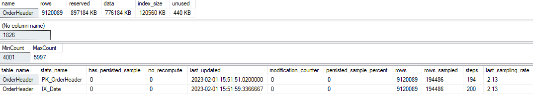
In this scenario, there is a limited number of distinct values (184 distinct submitted dates – from July 2022 to December 2022) and the distribution of the data is relatively balanced (between 40’000 and 60’000 order headers per day):

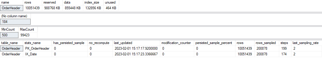
This will return something close to:

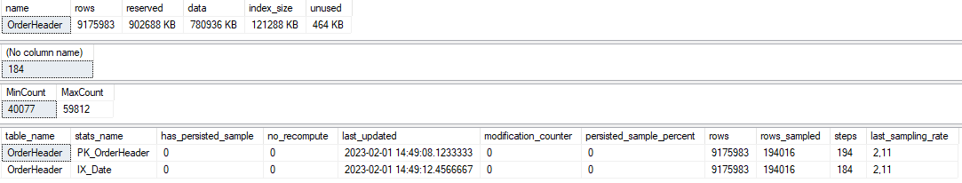
We can see that the statistics are up-to-date, and have been computed with a sampling rate of 2.11%. Then launch an analysis of the statistic:

It completes after a couple of seconds, and we can use column “log_details” in the last dataset returned to get the logs:

Based on this synthesis, we can see that all the steps are “compliant” with the thresholds used for

And as we have passed the value 1 to the parameter @p_ShowDetails of the stored procedure, we can use the histogram dataset returned by the stored procedure to build a representation:

 

The X axis represents the histogram steps, the Y axis represents the value of the factor of difference and the value of the coefficient of variation. So, with the default value of 10 for @p_MaxDifferenceFactor and 1000 for @p_MaxCov, we can confirm that all the steps are “compliant” with the thresholds used:

• the difference factor for equal_rows, obtained by considering the greatest value between [equal_rows estimated divided by equal_rows actual] and [equal_rows actual divided by equal_rows estimated] fluctuates between 1 and less than 4, which makes sense as the distribution of the data is quite linear
• the difference factor for average_range_rows, obtained by considering the greatest value between [average_range_rows estimated divided by average_range_rows actual] and [average_range_rows actual divided by average_range_rows estimated] is always 1, which makes sense as the ranges are empty (value set to 1 by StatMan, not 0)
• the coefficient of variation is always 0, because the ranges are empty

Knowing that we are in scenario 1, which is based on the easiest data pattern to deal with, it is not surprising to get these results with just the default sampling rate. The estimates based on this statistic will be extremely accurate, so we are good and we can move on to the next scenario.

Scenario 2

In this scenario, there is a limited number of distinct values (184 distinct submitted dates – from July 2022 to December 2022) and the distribution of the data is not balanced (between 1 and 100’000 order headers per day):

We can see that the statistics are up-to-date, and have been computed with a sampling rate of 2%. Then launch an analysis of the statistic and review the logs:

Based on this synthesis, we can see that this time some steps are not “compliant” with the thresholds used for

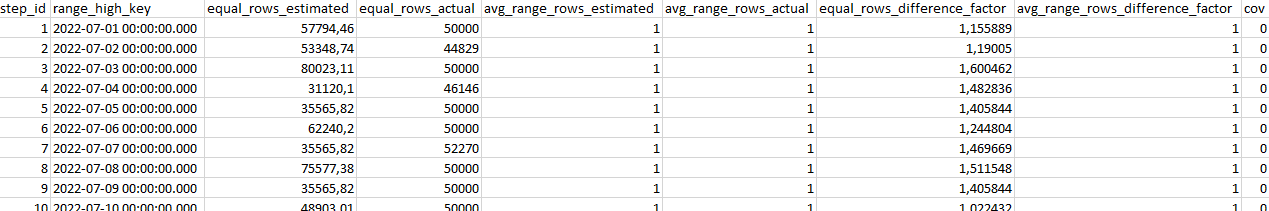
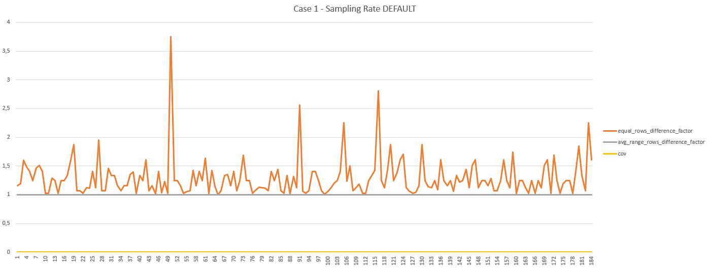
Let’s use histogram dataset returned by the stored procedure to figure out which steps are not compliant (because of average_range_rows_difference_factor AND coefficient of variation) and correlate this with the logs:

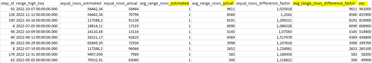
As we can see, for these steps the average_range_rows estimated is 1, meaning on average 1 order header submitted per day on the days that are part of the range. But actually, there have been on average between 500 and 9611 order headers submitted per day on the days that are part of the range. In this scenario it looks like StatMan did not detect the order headers that have been submitted on the days that are part of these ranges.

And indeed, the probability to miss out dates where only a few thousands of order headers have been submitted is high as that there may be days with up to 100’000 order headers submitted and that the sampling is low, at 2%.

Let’s check for instance on the 6th of October 2022:

The actual plan for this query is:

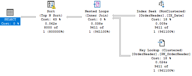
Looking at the execution plan, we can confirm the estimation was completely wrong, and we get a spill on the sort operator as not enough memory was requested / granted. Of course, the performance impact is limited on such simple queries, but as the complexity of the query grows (e.g. joins with multiple other large tables) it may become a serious problem. And if a plan based on such estimates is cached and reused by subsequent executions of the same code / stored procedure, it may impact multiple processes and users.

So, would a higher sampling rate help in this scenario? Let’s figure out by calling the stored procedure with the parameter @p_TryTuning set to 1:

And get the logs:

We can notice that there have been 3 rounds to assess tuning opportunities:

• the initial round, with the default sampling rate and the results we already know

{“round_id”:1,”steps”:174,”sampling_rate”:2,”is_default”:1,”steps_exceeding_difference_factor”:10,”steps_exceeding_cov”:10,”round_duration_ms”:2110}

• a second round, with a sampling rate of 10%, led to a drop (from 10 to 1) of the number of steps not compliant with the thresholds

• a third round, with a sampling rate of 20%, led to the removal of all the steps not compliant

As the results obtained with a sampling rate of 20% led to the removal of all the steps not compliant, the optimization process stopped and considered that the optimal sampling rate is 20%.

Scenario 3

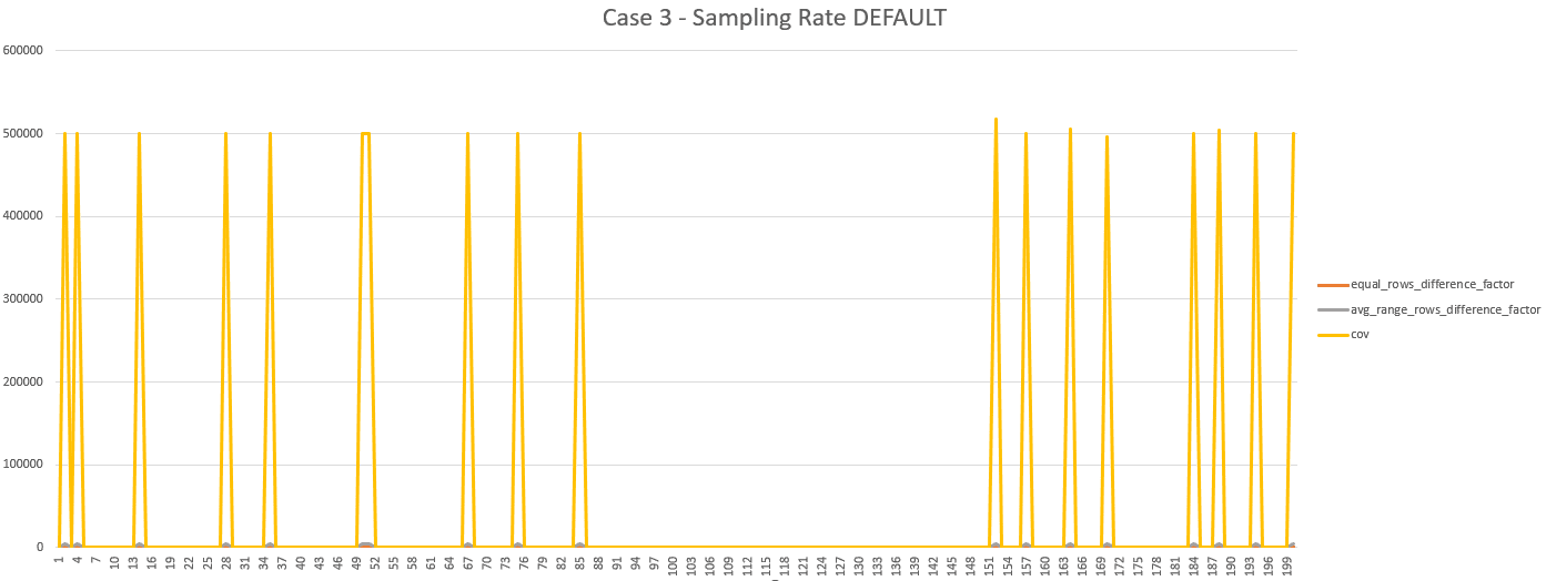
In this scenario, there is a large number of distinct values (1826 distinct submitted dates – from January 2018 to December 2022) and the distribution of the data is relatively balanced (between 4’000 and 6’000 order headers per day):

We can see that the statistics are up-to-date, and have been computed with a sampling rate of 2.13%. Then launch an analysis of the statistic with tuning attempt and review the logs:

We can notice that there have been 4 rounds to assess tuning opportunities:

• the initial round, with the default sampling rate and 18 steps not compliant with the thresholds

The explanation is similar to scenario 2 “…StatMan did not detect the order headers that have been submitted on the days that are part of these ranges.” but the root cause is slightly different: the probability to miss out dates is high because there are a lot of distinct dates and that the sampling is quite low, at 2.13%.

• a second round, with a sampling rate of 10%, that led to a drop (from 18 to 5) of the number of steps not compliant with the thresholds

{"round_id":2,"steps":189,"sampling_rate":10,"is_default":0,
"steps_exceeding_difference_factor":5,"steps_exceeding_cov":5,
"round_duration_ms":8843}

• a third round, with a sampling rate of 20%, led to another drop (from 5 to 3) of the number of steps not compliant with the thresholds

{"round_id":3,"steps":191,"sampling_rate":20,"is_default":0,
"steps_exceeding_difference_factor":3,"steps_exceeding_cov":3,
"round_duration_ms":10267}

• a fourth round, with a sampling rate of 30, led to the removal of all the steps not compliant

{"round_id":4,"steps":198,"sampling_rate":30,"is_default":0,
"steps_exceeding_difference_factor":0,"steps_exceeding_cov":0,
"round_duration_ms":10803}

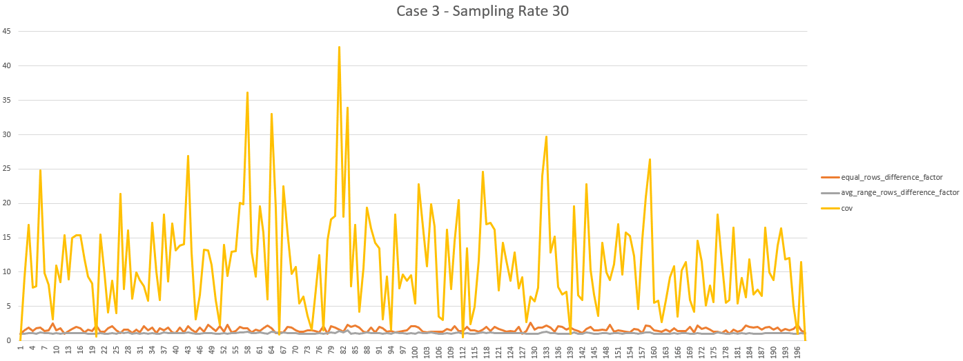
As the results obtained with a sampling rate of 30% led to the removal of all the steps not compliant, the optimization process stopped and considered that the optimal sampling rate is 30%.

Scenario 4

In this scenario, there is a large number of distinct values (1826 distinct submitted dates – from January 2018 to December 2022) and the distribution of the data is not balanced (between 1 and 100’000 order headers per day):

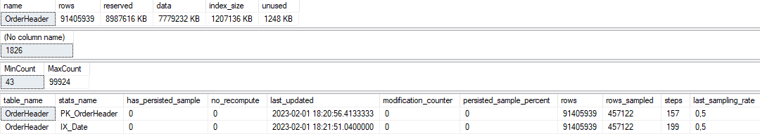
We can see that the statistics are up-to-date, and have been computed with a sampling rate of 0.5%, which is lower than in the previous scenarios as the table is larger (around 8 GBs). Then launch an analysis of the statistic with tuning attempt and review the logs:

We can notice that there have been 2 rounds to assess tuning opportunities:

• the initial round, with the default sampling rate and 9 steps not compliant with the thresholds

{"round_id":1,"steps":199,"sampling_rate":0.5,"is_default":1,
"steps_exceeding_difference_factor":9,"steps_exceeding_cov":8,
"round_duration_ms":19776}

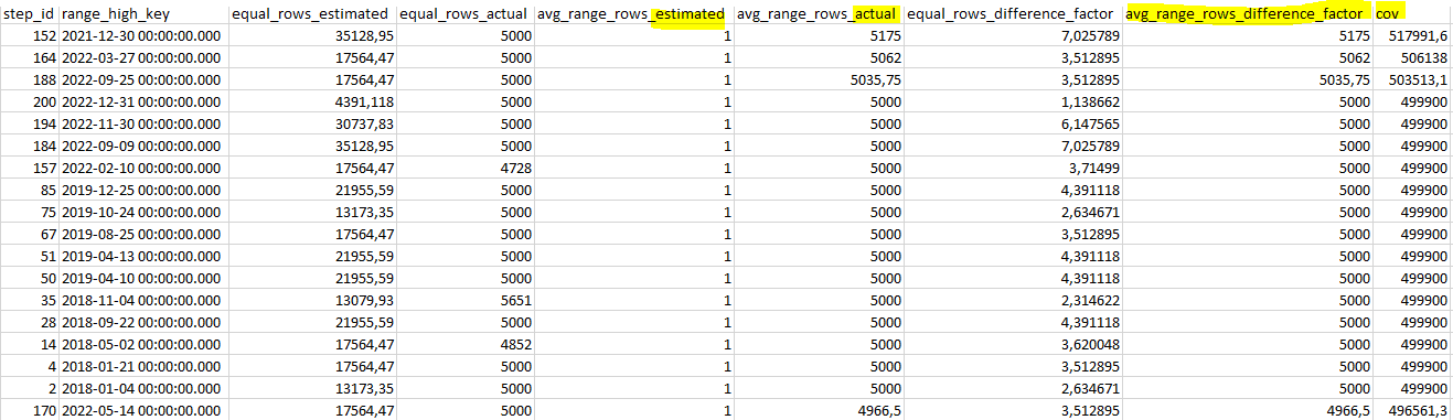
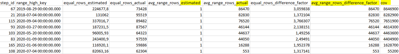
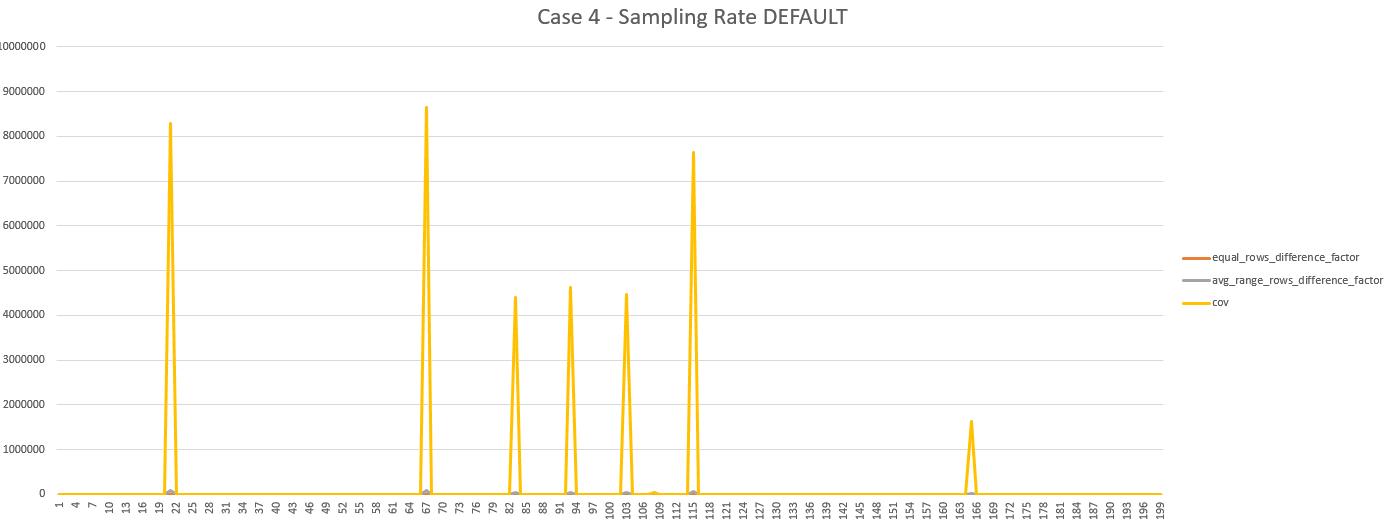
Let’s use the histogram dataset returned by the stored procedure to investigate a bit more, by sorting the data by avg_range_rows_difference_factor (descending):

• a second round, with a sampling rate of 10%, led to an increase (from 9 to 23) of the
• |

{"round_id":1,"steps":199,"sampling_rate":0.5,"is_default":1,
"steps_exceeding_difference_factor":9,"steps_exceeding_cov":8,
"round_duration_ms":19776}

Let’s use the histogram dataset returned by the stored procedure to investigate a bit more, firstly by sorting the data by avg_range_rows_difference_factor (descending) to get the step exceeding the difference factor for this metric:

Secondly, we can sort the data by equal_rows_difference_factor (descending), to get the 22 steps exceeding the difference factor for this metric:

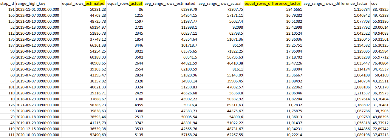
In this scenario, this metric should not be considered as an actual issue: as there may be up to 100’000 order headers per day, it is not that bad to build (and possibly cache) a plan for an estimated number of a couple of dozen of thousands of order headers.

Considering that there are 1826 distinct dates in the table, having this discrepancy on only 22 dates could safely be ignored. So, to conclude this scenario, the default sampling rate is likely to be enough, especially considering the size of the table (cost of maintaining the statistic).

What’s next?

Give it a try. Now that we have demonstrated a process to automate the analysis of statistics on synthetic data, you may want to evaluate the accuracy of statistics in your databases. Should you want to give it a try in your environment, please keep in mind that the methodology presented is usable at your own risks, without any guarantee.

With that disclaimer in mind, here is a skeleton of methodology you can follow:

• execute the stored procedure on a copy of a production database (preferably without data updates during the analysis), with @p_TryTuning=1 (e.g. on a server where you restore production backups on a regular basis to make sure that you can actually restore your backups)

Reminder: this stored procedure will update statistics

• review the result of the assessment with this query

Note: you can filter on “JSON_VALUE(log_details,'$.optimal_sampling_rate_is_default')<>'1‘” to list only the statistics for which a custom sampling rate has been identified

• still on your copy of the production database, activate the query store, execute a simulation of the production workload, deploy the custom sampling rates with the option PERSIST_SAMPLE_PERCENT=ON, re-execute the workload and compare the results (e.g. query performance, resource usage)

WARNING: updating statistics does not guarantee that the execution plan(s) relying on these tables / statistics will be recompiled. Typically, if the modification counter is 0 when the statistics are updated, it won’t cause a recompile. It is however possible to force a recompilation of the plans relying on a table by calling sp_recompile with the table name as parameter.

• to evaluate the gains with the custom sampling rate, the most reliable technique is to use the query store and limit the scope of the analysis to the query having execution plans relying on the statistics that have been modified (available in the execution plans since SQL 2017 and SQL 2016 SP2 with the new cardinality estimator – see SQL Server 2017 Showplan enhancements)
• to evaluate the overhead of the custom sampling rate you can:
  • (on production) monitor the automatic updates on these statistics over a period of time using an Extended Event (XE) session to capture the events “sqlserver.auto_stats” (filter by table and statistic if needed)
  • on your copy of the production database, start an Extended Event (XE) session to capture the events “sqlserver.sql_statement_completed” reporting the IOs/CPU consumed with the default sampling rate and with the custom sampling rate (using UPDATE STATISTICS command)
  • compute the overhead of the custom sampling rate ([cost with custom sampling rate – cost with default sampling rate])
  • multiply the overhead of the custom sampling rate by the number of automatic updates that have been identified by the XE session, plus the number of updates that are triggered explicitly by the application and IT maintenance scripts
  • (on production), compare the overhead obtained with the cost of all the queries (use sys.query_store_runtime_stats, filtered on the period of time where you have monitored the automatic updates of statistics)

Note: this technique will only give you an indication, not a guarantee (e.g. if the statistics updates occur on a timeframe where you server capacity is almost saturated, updating with a higher sampling rate during this timeframe could create more problems than it may solve)

• (on production) deploy the custom sampling rates using the UPDATE STATISTICS command with the option PERSIST_SAMPLE_PERCENT=ON and after a period of time compare the results (see above)

Lastly, whatever the methodology that you choose, make sure to document your tests and the changes implemented. It will make your life easier to explain it / do a handover and you may want to re-assess these changes after a period of time (e.g. as the database grows or shrinks over time). And of course, keep me posted when you find bugs or improvements 🙂

Other options

Sometimes, you may find out that statistics are the root cause of significant discrepancies between the estimates and the actuals leading to the creation (and possibly caching) of poorly performing execution plans, but unfortunately increasing the sampling rate is not possible (e.g. too costly) or it does not help much (depending on the data pattern). In such situations, there are a couple of options that you may consider:

• filtered statistics, filtered indexes and partitioned views (each underlying table has its own statistics) may come in handy to “zoom” on some ranges of data (spoiler alert: they come with some pitfalls, see the presentation by Kimberley L. Tripp)
• archiving data in another table and purging data are also valid options that could be helpful for maintenance and statistics accuracy; restricting the number of rows “online” is likely to lead to a higher (and more stable) sampling rate and the number of distinct values to model in the histogram steps may be reduced as well
• partitioning will primarily help for maintenance if you use incremental statistics (not enabled by default), but the estimates will still be derived from a merged histogram that covers the whole table (see this excellent article from Erin Stellato); this is one of the reasons why you may prefer partitioned views
• the sampling rate is primarily based on the table size, so if enabling compression (row or page) reduces the number of pages, then the default sampling rate may increase; similarly, the fill factor also impacts the number of pages (the lower it is, the higher the sampling rate may be)

Intelligent Query Processing

SQL Server Intelligent Query Processing (IQP) is a set of features that have been introduced progressively, and some of them may help to mitigate incorrect estimations (and not only the ones extrapolated from the statistics). We will not detail them (Erik Darling and Brent Ozar have already explained a lot of details – and pitfalls!) but it is important to mention them and keep them in mind when evaluating the update of your SQL services. Starting with SQL 2017:

• Adaptive Joins (Batch Mode)
• Interleaved Execution (with multi-statement table valued function)
• Memory grant feedback (Batch Mode)

Then SQL 2019 added another set of features:

• Memory grant feedback (Row Mode)
• Table Variable Deferred Compilation (which was somehow mitigated in previous versions with trace flag 2453)

And more recently with SQL 2022:

• Cardinality estimation feedback (CE feedback)
• Memory grant feedback (Percentile)
• Memory Grant, CE and DOP feedback persistence
• Parameter Sensitive Plan Optimization (PSPO) (which interestingly relies directly on statistics!)

These features are great improvements that contribute to the popularity of SQL Server in the relational database engines market, and they will most likely be improved and enriched over time. However, I believe that we should not rely solely on these kinds of improvements (or trace flags, hints, plan guides, query store plan forcing and so on) to fix estimation issues.

Conclusion

In this article, we have discussed the concept of “statistics accuracy”, which is relative and depends on multiple factors, then the main factors that affect statistics accuracy and we have demonstrated a process to automatically evaluate and, when possible, tune statistics.

The key takeaway is that the data pattern has a major impact on the accuracy of the statistics, and you can relatively easily modify the sampling rate, the frequency of the statistics updates, use hints and trace flags, but it is much more challenging to act upon the data and its modelisation (e.g. with partitioned views, archiving, purging) to increase statistics accuracy. It is also important to keep in mind that some changes may require modifications of the workload / applications to be leveraged (e.g. filtered statistics, filtered indexes or partitioned views).

The good news is, if you are actually facing issues related to estimations, that there are solutions, and some of them are delivered out of the box with modern versions of SQL Server. Additionally, you can investigate on your own systems with the methodology suggested, so you may gain some useful insights about your statistics. Finally, I hope that you found this article interesting, and that you have learned something!