The series so far:

1. Power BI Introduction: Tour of Power BI — Part 1
2. Power BI Introduction: Working with Power BI Desktop — Part 2
3. Power BI Introduction: Working with R Scripts in Power BI Desktop — Part 3
4. Power BI Introduction: Working with Parameters in Power BI Desktop — Part 4
5. Power BI Introduction: Working with SQL Server data in Power BI Desktop — Part 5
6. Power BI Introduction: Power Query M Formula Language in Power BI Desktop — Part 6
7. Power BI Introduction: Building Reports in Power BI Desktop — Part 7
8. Power BI Introduction: Publishing Reports to the Power BI Service — Part 8
9. Power BI Introduction: Visualizing SQL Server Audit Data — Part 9

Power BI Desktop provides a far more robust environment for developing business intelligence reports than the Power BI service. Power BI Desktop supports more data sources and offers more tools for transforming the data retrieved from those sources.

One data source available to Power BI Desktop that is not available to the service is SQL Server. Although the Power BI service provides connectors to Azure SQL Database and SQL Data Warehouse, it does not offer one for SQL Server. With Power BI Desktop, you can retrieve SQL Server data from entire tables or run queries that return a subset of data from multiple tables. You can also call stored procedures, including the sp_execute_external_script stored procedure, which allows you to run Python and R scripts.

This article walks you through the process of retrieving data from a SQL Server instance, using different methods for returning the data. The article also covers some basic transformations. The examples are based on the AdventureWorks2017 database, running on a local instance of SQL Server, but the principles apply to any SQL Server database.

In fact, many of the topics covered here can apply to other relational database management systems and even other types of data sources. Because Power BI Desktop organizes all data into queries (table-like structures for working with datasets), once you get the data into Power BI Desktop, many of the actions you carry out are similar despite the source. That said, you’ll still find features specific to relational databases, particularly when it comes to the relationships between tables.

Retrieving SQL Server Tables

In Power BI Desktop, you can retrieve SQL Server tables or views in their entirety. Power BI Desktop preserves their structures and, where possible, identifies the relationships between them. This section provides an example that demonstrates how importing tables works. If you follow along, you’ll start by retrieving three tables from the AdventureWorks2017 database.

To retrieve the tables, click Get Data on the Home ribbon in the main Power BI Desktop window. When the Get Data dialog box appears, navigate to the Database category and double-click SQL Server database. In the SQL Server database dialog box, provide the name of the SQL Server instance and the target database, as shown in the following figure.

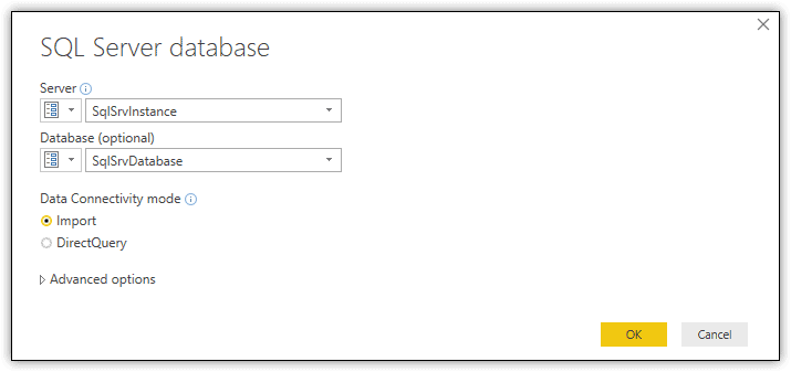
For this article, I created two connection parameters. The first parameter, SqlSrvInstance, contains the name of the SQL Server instance. The second parameter, SqlSrvDatabase, contains the name of the database. When providing the connection information, you can use the actual names or you can create your own parameters. For details about creating parameters, refer to the previous article in this series.

Once you’ve entered the necessary information, click OK. When the Navigator dialog box appears, select the Person.Address, Person.BusinessEntityAddress, and Person.Person tables, as shown in the following figure.

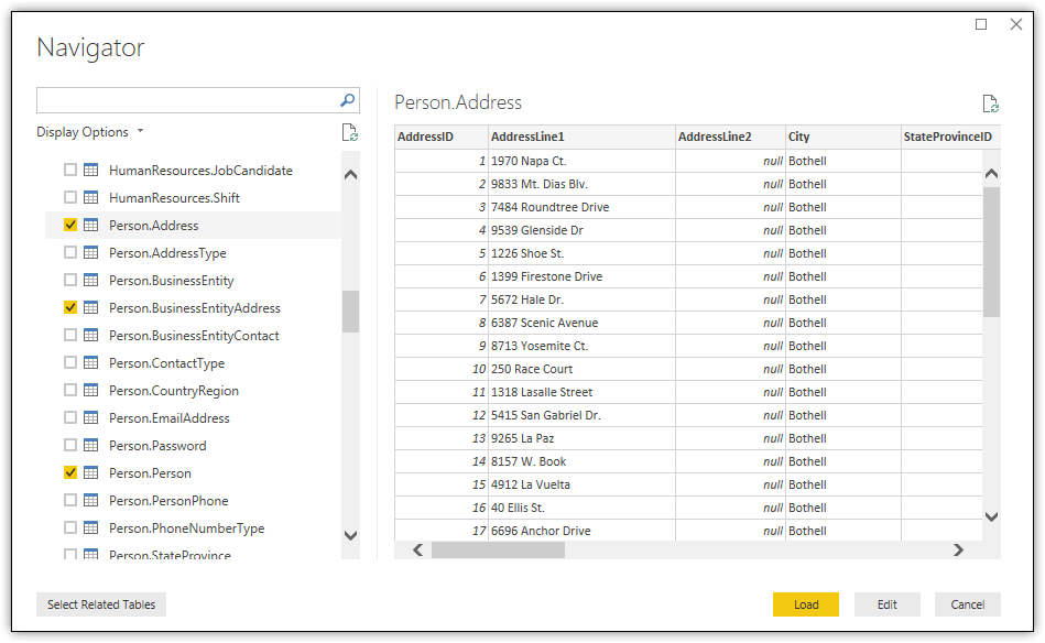
You can review the data from the selected table in the right pane. You can also choose to include related tables by clicking the Select Related Tables button. For example, if you select the Person table and then select the related tables, you would end up with nine tables, a lot more than you need for this example. Whether you take advantage of this option will depend on your specific project. If you do, but don’t want to keep all the selected tables, simply clear the checkboxes associated with those you want to exclude.

When you’re ready to import the tables into Power BI Desktop, click the Load button. Any tables and views you’ve selected will be loaded into Power BI Desktop and listed as individual datasets in Data view. From there, you can modify the datasets in Query Editor, just as you would data retrieved from any other source.

One of the first steps you’re likely to take in Query Editor is to rename each dataset and from there, remove any extra columns:

• To rename a dataset, right-click the dataset in the Queries pane, click Rename, type in the new name, and press Enter.

• To remove a column, select the column in the main grid and click Remove Columns on the Home ribbon.

• To remove multiple columns in one operation, select the first column, press and hold Control as you select each additional column, and then click Remove Columns on the Home ribbon.

With these instruction in mind, take the following steps for the three tables you just imported:

• Change the name of the Person Address table to Address, and then remove the columns AddressLine1, AddressLine2, PostalCode, SpatialLocation, rowguid, and ModifiedDate.

• Change the name of the Person BusinessEntityAddress table to BusEntAddress, and then remove the columns AddressTypeID, rowguid, and ModifiedDate.

• Change the name of the Person Person table to Person, and then remove the columns PersonType, NameStyle, Title, MiddleName, Suffix, EmailPromotion, AdditionalContactInfo, Demographics, rowguid, and ModifiedDate.

For now, ignore the columns that contain relationship data (the columns with the gold-colored values). We’ll get back to those shortly.

When you’re finished updating the queries, apply your changes and close Query Editor. Your datasets should look like those shown in the following figure, as they appear in Data view. In this case, the Person dataset is selected.

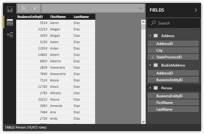
Notice that each dataset now includes only two or three fields. You can also add filters in Query Editor to refine the data even more, or you can add filters to individual visualizations when you’re building your reports.

Working with Relationships

When you updated your datasets in Query Editor, you no doubt noticed that the queries included a number of pseudo-columns, indicated by the long column names and gold-colored values, which are either Table or Value.

The columns reflect the relationships that exist between the between tables in the source database. A column that contains Table values represents a foreign key in another table that references the primary table on which the query is based. A column that contains Value values represents a foreign key in the primary table that references another table.

For example, when you select the Address query in Query Editor, you should see four relationship columns, as shown in the following figure.

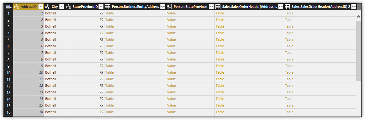
The columns indicate that the Address table, as it exists in the AdventureWorks2017 database, contains one foreign key and is referenced by three foreign keys:

• The Person.BusinessEntityAddress column in the Address query represents a foreign key in the Person.BusinessEntityAddress table that references the Person.Address table. The key is created on the AddressID column in the Person.BusinessEntityAddress table.

• The Person.StateProvince column in the Address query represents a foreign key in the Person.Address table that references the Person.StateProvince table. The key is created on the StateProvinceID column in the Person.Address table.

• The Sales.SalesOrderHeader(AddressID) column in the Address query represents a foreign key in the Sales.SalesOrderHeader table that references the Person.Address table. This key is created on the BillToAddress column in the Sales.SalesOrderHeader table.

• The Sales.SalesOrderHeader(AddressID) 2 column in the Address query represents a foreign key in the Sales.SalesOrderHeader table that references the Person.Address table. This key is created on the ShipToAddress column in the Sales.SalesOrderHeader table.

If you click a Value or Table value, Query Editor will add a step to the Applied Steps section in the right pane and modify the dataset to include information specific to the selected value. For example, the first row in the Address query contains an AddressID value of 1 and a StateProvinceID value of 79. If you click the Value value in the Person.StateProvince column for that row, Query Editor will add a step named 1 to Applied Steps and modify the dataset to include only information from the StateProvince table specific to the StateProvinceID value of 79, as shown in the following figure.

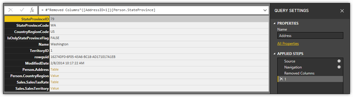
You can click any instance of Value in the Person.StateProvince column to see the related data. The associated step in the Applied Steps section will be named after the AddressID value of the selected row. When you are finished viewing the results, you can return the query to its previous state by deleting the added steps in the Applied Steps section.

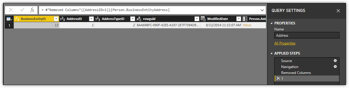
If you were to now click the Table value in the Person.BusinessEntityAddress column for the first row, Query Editor would again add a step named 1, only this time the information would come from the BusinessEntityAddress table, and the modified dataset would include only one row, as shown in the following figure. The row includes a foreign key reference to the AddressID value of 1 in the Address table.

You can play with the Value and Table values as much as you like to see the different related data. Just be sure to remove the step from Applied Steps to return the query to its previous state. Although you won’t be using this feature for the examples in this article, you might find it useful for other projects based on SQL Server data.

In addition to identifying foreign key relationships, Power BI Desktop also attempts to identify the relationships between the imported datasets. You can view these relationships by going to the Relationships pane in the main Power BI Desktop window. There you’ll find a graphically representation of each dataset, which you can move around as necessary. If Power BI Desktop detects a relationship between two datasets, they’re joined by a connector that indicates the type of relationship, as shown in the following figure.

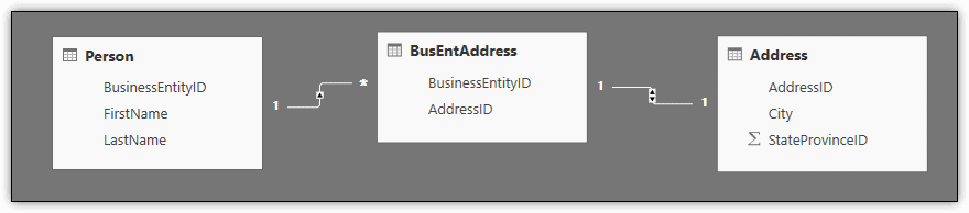
In this case, Power BI Desktop has detected a one-to-many relationship between the Person and BusEntAddress datasets and a one-to-one relationship between the BusEntAddress and Address datasets. You can view details about a relationship by double-clicking the connector. For example, to view details about the relationship between the Person and BusEntAddress datasets, double-click the connector that joins the datasets. This launches the Edit relationship dialog box, shown in the following figure.

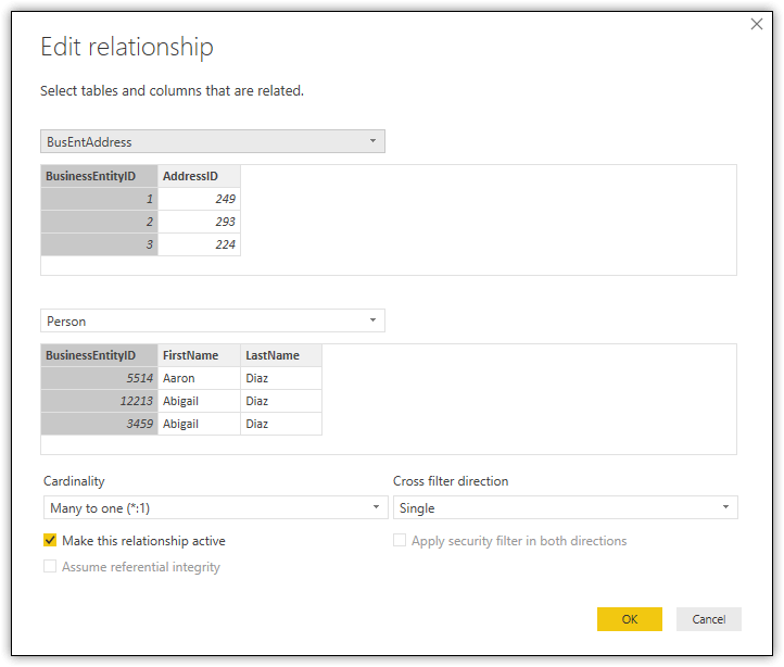
In the dialog box, you can view the details about the relationship and even modify them if necessary, although Power BI Desktop does a pretty good job at getting the relationships right, based on the current data in the dataset. Notice that the dialog box shows this as a many-to-one relationship, rather than one-to-many. This is because the BusEntAddress dataset is listed first. You can find details about defining and editing relationships, as well as the meaning of the individual options, in the Microsoft article Create and manage relationships in Power BI Desktop.

The fact that Power BI Desktop detects relationships makes it easier to create visualizations based on multiple datasets. For example, I created a simple table visualization in Report view based on data from the Person and Address datasets, without having to map data across all three datasets. The following figure shows the table with a filter applied on the visualization (the StateProvinceID value set to 1).

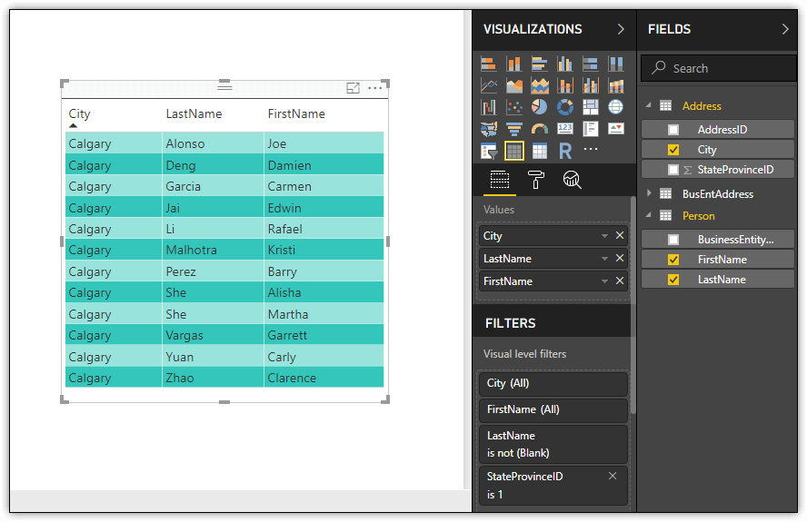
We’ll be digging into how to create visualizations in a later article in this series, so I won’t be going into any details here. Just know that relationships can make this process simpler because the data is mapped for you.

Merging Datasets

In some cases, you might want to combine multiple datasets into a single one. For example, you might decide to merge the three datasets you created earlier. To do so, open Query Editor and select the Person query. On the Home ribbon, click the Merge Queries down arrow and then click Merge Queries as New.

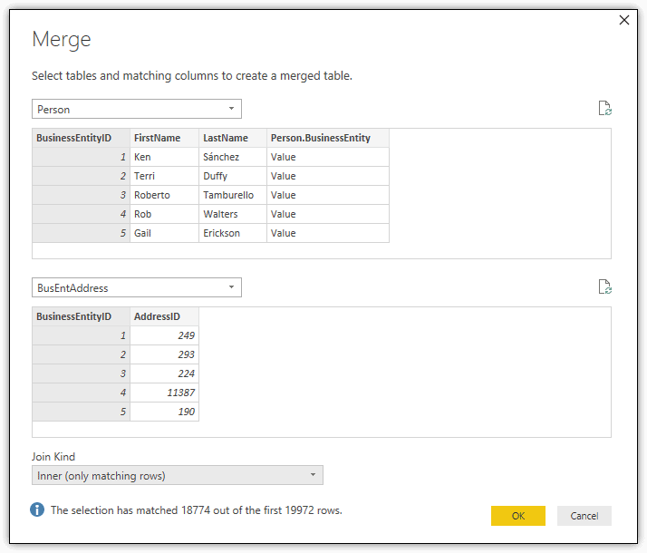
In the Merge dialog box (shown in the following figure), verify that the Person dataset is selected in the first drop-down list. Next, select BusEntAddress from the second (middle) drop-down list, and then select Inner (only matching rows) from the Join Kind drop-down list. This tells Query Editor to create an inner join between the two queries. Then, for each referenced dataset, select the BusinessEntityID column and click OK.

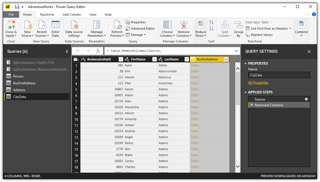
When you click OK, Query Editor creates a new query, which you can rename CityData. The CityData query contains the three primary columns from the Person dataset, along with a number of relationship columns. Delete all the relationship columns except the last one, BusEntAddress, which represents the BusEntAddress query. Your merged query should now look like the one shown in the following figure.

The next step is to select one or more columns from the BusEntAddress query to add to the merged query. To select the columns, click the icon at the top right corner of the BusEntAddress column and clear all but the AddressID column, as shown in the following figure. You do not need to add the BusinessEntityID column because it is already included in the Person dataset, and the other columns are relationship columns.

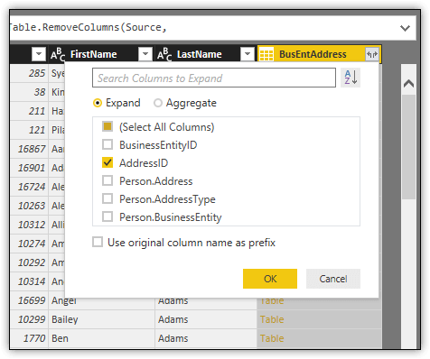
Also clear the Use original column name as prefix checkbox to keep the column name simple, and then click OK. The CityData query will now include the AddressID column.

The next step is to merge the Address query into the CityData query. With the CityData query still selected in Query Editor, click the Merge Queries button on the Home ribbon. In the Merge dialog box (shown in the following figure), select Address from the second drop-down list and select Inner (only matching rows) from the Join Kind drop-down list. For each data set, select the AddressID column and then click OK.

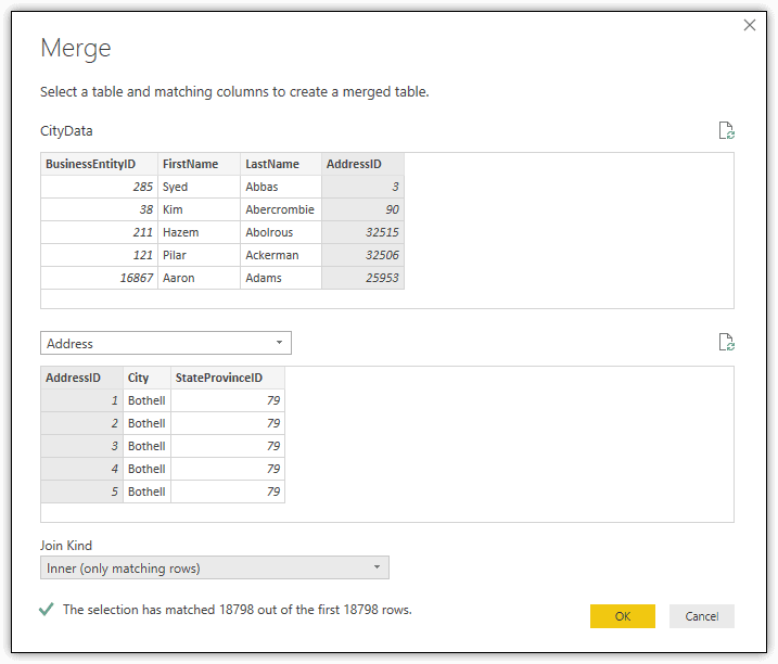
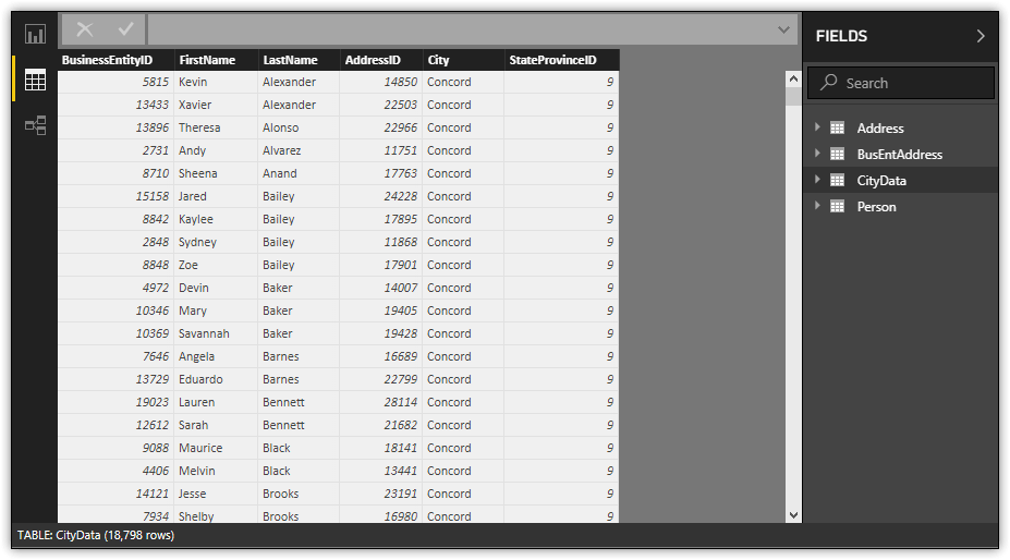
Next, click the icon at the top right corner of the Address reference column and clear all but the City and StateProvinceID columns. Also clear the Use original column name as prefix checkbox, if selected, and then click OK. Your merged dataset should now look like the one in the following figure.

With the merged query in place, you have a single dataset from which you can perform other operations. For example, you can apply additional transformations such as pivoting data, splitting columns, or filtering rows, while still preserving the original datasets. A single dataset can also make it easier create visualizations because you don’t have to navigate multiple sources. Like any feature in Power BI Desktop, your specific requirements will determine whether you can benefit from merged queries.

Using T-SQL Queries to Retrieve SQL Server Data

Although you can transform data in a variety of ways in Power BI Desktop, one of the most powerful tools you have at your disposal is the ability to use T-SQL queries to return data from a SQL Server database, rather than specifying individual tables or views. With a query, you can retrieve exactly the data you want, without having to remove columns, filter rows, or take other steps after importing the data. In this way, you’re working with a single dataset that includes exactly the data you need, rather than trying to navigate multiple datasets that contain a lot of data you don’t want.

In the next example, you’ll use the following SELECT statement to join together six tables in the AdventureWorks2017 database and return the data to Power BI Desktop:

To run the query, click Get Data on the Home ribbon in the main Power BI Desktop window. When the Get Data dialog box appears, navigate to the Database category and double-click SQL Server database.

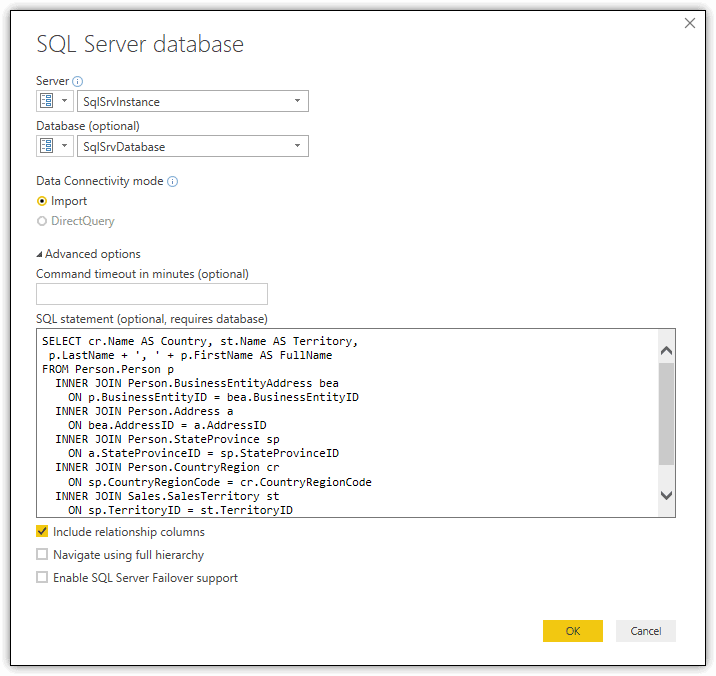
In the SQL Server database dialog box, provide the name of the SQL Server instance and the target database and then click the Advanced options arrow, which expands the dialog box. In the SQL statement box, type or paste the above SELECT statement, as shown in the following figure.

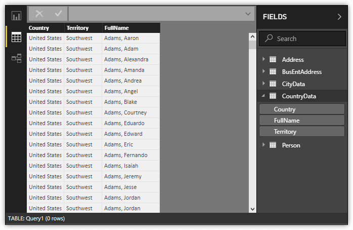
When you click OK, Power BI Desktop displays a preview window, showing you a subset of the data you’ll be importing. Click Load to import the data into Power BI Desktop. After the data has loaded, go to Data view, right-click the new dataset, and then click Rename. Type CountryData and press Enter. The new dataset should look similar to the one shown in the following figure.

Now you have the dataset exactly as you need it, without all the extra steps that come with importing individual tables. You can still apply additional transformations if necessary, but often that will not be needed.

In Power BI Desktop, you can run a wide range of T-SQL queries when retrieving data from a SQL Server database, including EXECUTE statements that call stored procedures. For example, you can call the sp_execute_external_script stored procedure in order to run an R script (SQL Server 2016 or later) or Python script (SQL Server 2017 or later), as shown in the following example:

In this case, the sp_execute_external_script stored procedure is running a Python script that identifies anomalies in a sample dataset containing iris flower data. I based this example on one in a previous article I wrote, SQL Server Machine Learning Services – Part 4: Finding Data Anomalies with Python, which is part of a series on Python in SQL Server. Refer to that article for a full explanation of how this statement works.

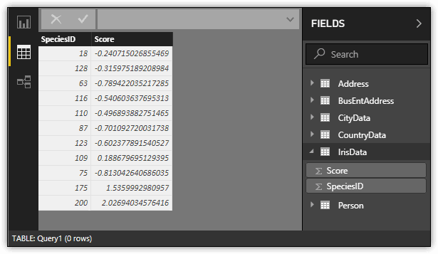
If you run this script, you should end up with the dataset similar to the one shown in the following figure, renamed to IrisData. (Because you’re working with random data, the values will usually be different each time you run the query.) The dataset includes the IDs used to identify iris species and scores that help to determine anomalies in the data.

Although this example does not include SQL Server data, it demonstrates that you can run a Python script from Power BI Desktop. You can also create a script that includes SQL Server data or data from multiple sources, opening up an even wider range of possibilities for pulling data into Power BI Desktop.

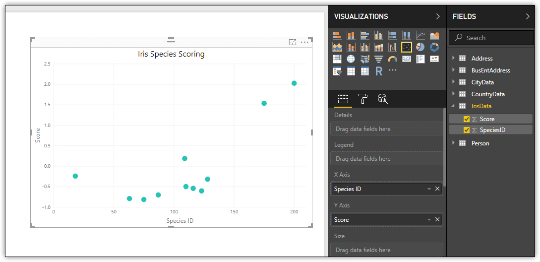
Best of all, you can take advantage of Python’s analytical capabilities, while importing the data in exactly the format you need, allowing you to easily create visualizations that provide critical insights into the available information. For example, I created a Scatter chart visualization based on this IrisData dataset, as shown in the following figure. Notice the two points in the chart toward the upper right corner. These represent the anomalies identified by the Python script.

Making the Most of SQL Server Data

The ability to run T-SQL queries in Power BI Desktop gives you a powerful tool for accessing SQL Server data. Not only does this allow you to maximize the benefits of the SQL Server query engine, but also minimize the size of the datasets you import into Power BI Desktop, while reducing the number of transformations you have to perform.

Of course, you must understand how to use T-SQL in order to take this approach, but if you do—or can get someone who does—you’ll have a great deal of flexibility for working with SQL Server data. That said, even if you retrieve data on a table-by-table basis, you still have a number of effective tools for working with SQL Server data and preparing it for creating meaningful visualizations that can be posted to the Power BI service.

Although the Power BI service lets you retrieve data from a number of sources, it does not provide a data connector for SQL Server. Of course, you can export SQL Server data to a file and then import that file into the service, but you cannot connect directly from the service to SQL Server, despite the critical role that SQL Server continues to play in many of today’s organizations. The better you understand how to import and transform SQL Server data in Power BI Desktop, the more effectively you can visualize SQL Server data in a variety of ways.