
Executive Summary
Power Query M is the formula language that Power BI Desktop uses behind the scenes when you apply data transformations in the Power Query Editor. Each transformation step you perform in the UI generates an M expression in a let statement – a chain of named steps where each step builds on the previous one. This article demonstrates writing M expressions directly, building a complete data transformation pipeline on a CSV dataset (the Titanic passenger data): loading the file, removing an unwanted column, promoting the first row to headers, renaming columns, filtering out null values, replacing coded values with readable text, changing capitalisation, and adding a calculated column. Writing M directly gives you more control and portability than the UI alone.
The series so far:
- Power BI Introduction: Tour of Power BI — Part 1
- Power BI Introduction: Working with Power BI Desktop — Part 2
- Power BI Introduction: Working with R Scripts in Power BI Desktop — Part 3
- Power BI Introduction: Working with Parameters in Power BI Desktop — Part 4
- Power BI Introduction: Working with SQL Server data in Power BI Desktop — Part 5
- Power BI Introduction: Power Query M Formula Language in Power BI Desktop — Part 6
- Power BI Introduction: Building Reports in Power BI Desktop — Part 7
- Power BI Introduction: Publishing Reports to the Power BI Service — Part 8
- Power BI Introduction: Visualizing SQL Server Audit Data — Part 9
In Power BI Desktop, a dataset is defined by a single query that specifies what data to include and how to transform that data. The query is made up of related steps that build on each other to produce the final dataset. Once you’ve defined the dataset, you can use it to create visualizations that you add to your reports, which you can then publish to the Power BI service.
At the heart of the query is the Power Query M formula language, a case-sensitive, data mashup language available to Power BI Desktop, Power Query in Excel, and the Get & Transform import feature in Excel 2016. As with many languages, Power Query statements are made up of individual language elements such as functions, variables, expressions, and primitive and structured values that together define the logic necessary to shape the data.
Each query in Power BI Desktop is a single Power Query let expression that contains all the code elements necessary to define a dataset. A let expression is made up of a let statement and an in statement, as shown in the following syntax:
|
1 2 3 4 |
let <em>variable</em> = <em>expression</em> [,...] in <em>variable</em> |
The let statement includes one or more procedural steps that define the query. Each step is essentially a variable assignment that consists of a variable name and an expression that provides the variable’s value. The expression defines the logic for adding, removing, or transforming the data in a specific way. This is where you’ll be doing the bulk of your work, as you’ll see in the examples to follow.
The variable can be of any supported Power Query type. Each variable within a let expression must have a unique name, but Power Query is fairly flexible about what you call it. You can even include spaces in the name, but you have to enclose it in double-quotes and precede it with a hash tag, a somewhat cumbersome naming convention (and one I prefer to avoid). The variable names are also the same names used to identify steps in the Applied Steps section in Query Editor’s right pane, so use names that make sense.
You can include as many procedural steps in your let statement as necessary and practical. If you include multiple steps, you must use commas to separate them. Each step generally builds on the preceding one, using the variable from that step to define the logic in the new step.
Strictly speaking, you do not have to define your procedural steps in the same physical order as their logical order. For example, you can reference a variable in the first procedural step that you define in the last procedural step. However, this approach can make the code difficult to debug and cause unnecessary confusion. The accepted convention when writing a let statement is to keep the physical and logical orders in sync.
The in statement returns a variable value that defines the dataset’s final shape. In most cases, if not all, this will be the last variable defined in your let statement. You can specify a different variable from the let statement, but there’s usually little reason to do. If you simply need to see a variable’s value at a specific point in time, you can select its related step in the Applied Steps section in Query Editor. When you select a step, you are essentially viewing the contents of the associated variable.
Retrieving Data from a CSV File
This article includes a number of examples that demonstrate how to define the procedural steps necessary to build a query. The examples are based on the titanic dataset available from this GitHub page. The titanic dataset lists the passengers on the infamous Titanic voyage and shows who survived and who did not. If you plan to try these examples for yourself, you need to create the titanic.csv file from the titanic dataset and save it to a folder that you can access from Power BI Desktop. On my system, I saved the file to my local folder C:\DataFiles\titanic.csv. There are several files named ‘titanic’ on the GitHub page, so be sure to download the Stat2Data Titanic file.
The first step in building your own Power Query script is to add a blank query to Power BI Desktop. To add the query, click Get Data on the Home ribbon in the main window, navigate to the Other section, and double-click Blank Query. This launches Query Editor with a new query listed in the Queries pane. The query is named Query1 or a similarly numbered name, depending on what queries you’ve already created.
To rename the query, right-click the query in the Queries pane, click Rename, type SurvivalLog, and press Enter. Then, on the View menu, click Advanced Editor. The editor will open with a new let expression defined, as shown in the following figure.
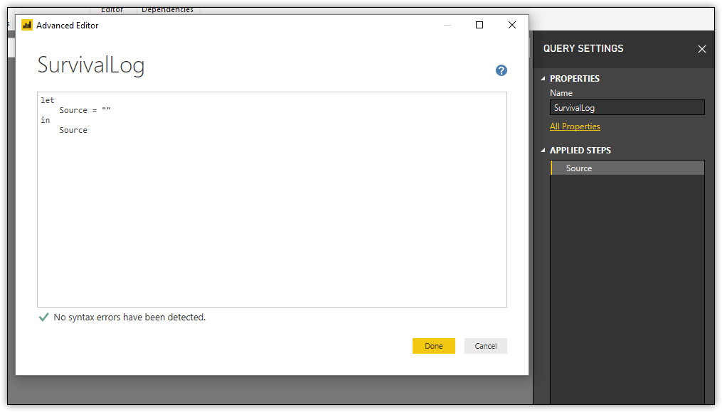
The let statement includes a single procedural step in which the variable is named Source and the expression is an empty string, as indicated by the double quotes. Notice that the variable is also listed in the in statement and as a step in the Applied Steps section of the right pane. For this exercise, you’ll be changing the variable name to GetPassengers.
The first procedural step that you’ll add will retrieve the contents of the titanic.csv file and save them to the GetPassengers variable. To add the procedure, replace the existing let expression with the following expression:
|
1 |
let GetPassengers = Csv.Document(File.Contents("C:\DataFiles\titanic.csv"), [Delimiter=",", Encoding=1252])in GetPassengers |
Notice that the GetPassengers variable is specified in the procedural step in the let statement and in the in statement. In this way, the variable’s value will be returned when the let expression runs.
The expression in the procedural step includes everything after the equal sign. The expression uses the Csv.Document function to retrieve the file’s contents as a Table object. The function supports several parameters, but only the first one is required to identify the source data. As part of the first parameter, you must also use the File.Contents function to return only the document’s data.
The second parameter can be specified as a record that contains optional settings. In Power Query, a record is a set of fields made up of name/value pairs enclosed in brackets. The record in this example includes the Delimiter and Encoding options and their values. The Delimiter option specifies a comma as the delimiter in the CSV document, and the Encoding option specifies the text encoding type of 1252, which is based on the Windows Western European code page.
That’s all there is to setting up a basic let expression. After you’ve entered your code, click Done to close the Advanced Editor and run the procedural step. The dataset, as it appears in Query Editor, should look similar to the following figure.
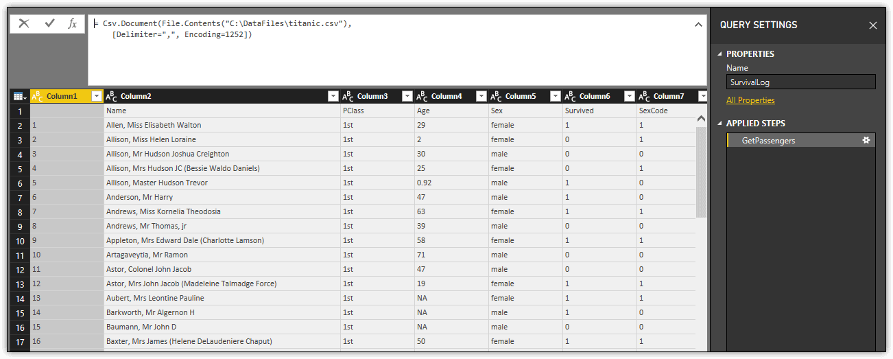
Notice that the first step in the Applied Steps section is named GetPassengers, the same as the variable name. The procedural step’s expression is also displayed in the small window above the dataset. You can edit the code directly in this window if necessary.
Whenever you add, modify, or delete a step, you should apply and save your changes. A simple way to do this is to click the Save icon at the top left corner of the menu bar. When prompted to apply your changes, click Apply.
Removing a Column from the Dataset
The next procedural step you will add to your let statement removes Column7 from the dataset. Because your dataset is saved as a Table object, you can choose from a variety of Power Query Table functions to update the data. For this step, you’ll use the Table.RemoveColumns function to filter out the specified column.
Click Advanced Editor to get back to the query. To remove the column, add a comma after the first procedural step and then, on a new line, define the next variable/expression pair, as shown in the following code:
|
1 |
let GetPassengers = Csv.Document(File.Contents("C:\DataFiles\titanic.csv"), [Delimiter=",", Encoding=1252]), RemoveCols = Table.RemoveColumns(GetPassengers, "Column7")in RemoveCols |
The Table.RemoveColumns function requires two parameters. The first parameter specifies the target table that you’ll be updating, which in this case, is the GetPassengers variable from the previous step. The second argument specifies a single column or a list of columns to be removed. This example specifies only Column7 from the GetPassengers table. The important takeaway here is how the second step builds on the first one and then returns a new result, which is assigned to the RemoveCols variable. The new variable contains the same dataset as the GetPassengers variable, less the Column7 data.
After you add the procedural step, replace the GetPassengers variable in the in statement with the RemoveCols variable. Next, click Done to close the Advanced Editor, and then save and apply your changes. You dataset should now look like the one shown in the following figure.
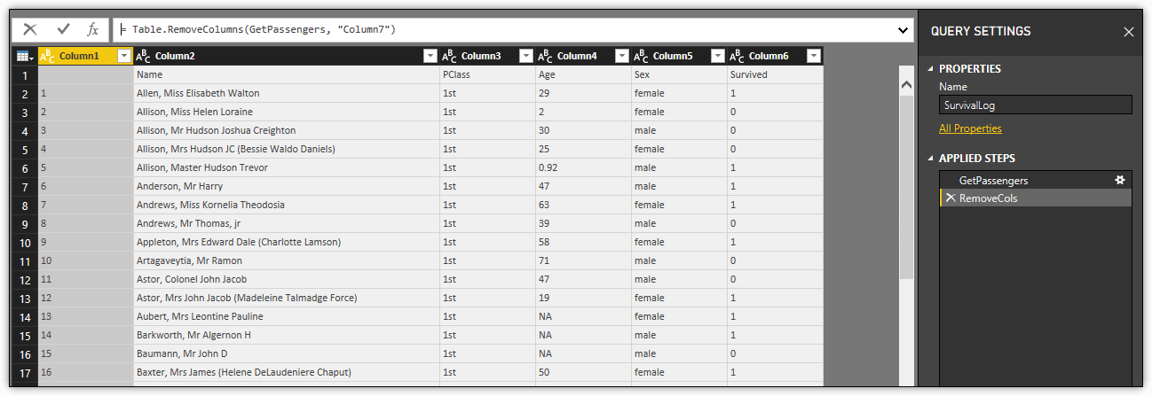
As you can see, the RemoveCols step has been added to the Applied Steps section and Column7 is no longer included in the dataset. To add more procedural steps, follow the same logic as here, continuing to build on your growing foundation.
Promoting the First Row to Headers
The next step is to promote the values in the first row of your dataset to the header row so these values become the column names. To carry out this step, add a comma after the last step you defined and then, on a new line, type the following variable/expression pair:
|
1 |
PromoteNames = Table.PromoteHeaders(RemoveCols, [PromoteAllScalars=true]) |
The expression uses the Table.PromoteHeaders function to promote the first row to the column headers. The function’s first parameter is required and specifies the table to use as the source data (the RemoveCols variable). This is just like you saw in the previous example, in which the new step builds on the previous step.
The second parameter, PromoteAllScalars, is optional, but is a good one to know about. By default, Power Query promotes only text and number values. When the PromoteAllScalars parameter is included and set to true, Power Query promotes all scalar values in the first row to headers.
The expression’s results are assigned to the PromoteNames variable. Be sure to update the in statement with this variable name.
Renaming Dataset Columns
Next, you will use the Table.RenameColumns function to rename several columns. The function returns a new Table object with the column names updated as specified. To rename the columns, add the following procedural step to your let statement, being sure to insert a comma after the previous statement:
|
1 2 |
RenameCols = Table.RenameColumns(PromoteNames, {{"", "PsgrID"}, {"PClass", "PsgrClass"}, {"Sex", "Gender"}}) |
The Table.RenameColumns function requires two parameters. The first is the name of the target table (the PromoteNames variable from the previous step), and the second is a list of old and new column names. In Power Query, a list is an ordered sequence of values, separated by commas and enclosed in curly brackets. In this example, each value in the list is its own list containing two values: the old column name and the new column name.
Filtering Rows in the Dataset
The next task is to filter out rows that contain NA in the Age columns and then filter out rows with Age values 5 or less. Because the Age column was automatically typed as Text when imported, you will need to filter the data in three steps, starting with the NA values. To filter out these values, add the following variable/expression pair to your code:
|
1 |
FilterNA = Table.SelectRows(RenameCols, each [Age] <> "NA") |
The Table.SelectRows function returns a table that contains only the rows that match the defined condition (Age not equal to NA). As you saw in the previous examples, the function’s first argument is target table, in this case, the RenameCols variable from the preceding step.
The second argument is an each expression specifying that the Age value must not equal NA. The each keyword indicates that the expression should be applied to each row in the target table. As a result, the new table, which is assigned to the FilterNA variable, will not include any rows with an Age value of NA.
Once you’ve remove the NA values, you should convert the Age column to the Number data type so you can work with the data more effectively, such as being able to filter the data based on a numerical age. When changing the type of the Age column, you can also change the type of the PsgrID column to the Int64 type. This way, you’re referencing the IDs by integers rather than text. To convert to the new data types, add the following variable/expression pair to the let statement:
|
1 2 |
ChangeTypes = Table.TransformColumnTypes(FilterNA, {{"PsgrID", Int64.Type}, {"Age", Number.Type}}) |
The expression uses the Table.TransformColumnTypes function to change the data types. The first parameter is the name of the target table (FilterNA), and the second parameter is a list of the columns to be updated, along with their new data types. Each value is its own list that includes the name of the column and type.
Once the Age column has been updated with the Number type, you can filter out the ages based on a numerical value, as shown in the following procedural step.
|
1 |
FilterKids = Table.SelectRows(ChangeTypes, each [Age] > 5) |
Your data set should now include only the desired data, as it exists in the FilterKids variable.
Replacing Column Values in a Dataset
Another handy transformation you might need to do at times is to replace one column value for another. For this example, you will replace the 0 value in the Survived column with No and the 1 value with Yes, using the Table.ReplaceValue function. To replace the 0 values, add the following procedural step to your code:
|
1 2 |
Replace0 = Table.ReplaceValue(FilterKids, "0", "No", Replacer.ReplaceText, {"Survived"}) |
The Table.ReplaceValue function requires the following five parameters:
- table: The target table, in this case, the variable from the preceding step.
- oldValue: The original value to be replaced.
- newValue: The value that will replace the original value.
- replacer: A Replacer function that carries out the replacement operation.
- columnsToSearch: The column or columns whose values should be replaced.
Most of the parameters should be self-explanatory, except perhaps the replacer parameter. For this, you can choose from several functions that work in conjunction with the Table.ReplaceValue function to update the values. In this case, the Replacer.ReplaceText function is used because text values are being replaced.
After you replace the 0 values, you can replace the 1 values with Yes, using the same construction:
|
1 |
Replace1 = Table.ReplaceValue(Replace0, "1", "Yes", Replacer.ReplaceText, {"Survived"}) |
Now the values in the Survived column are more readable for those who might not understand the meaning of the 0 and 1 values. It also makes it less likely that the data will cause any confusion.
Changing the Case of Column Values
Another way you can modify column values is to change how they are capitalized. For this example, you will update the values in the Gender column so the first letter is capitalized, rather than being all lowercase. To make these changes, add the following procedural step to the let statement:
|
1 |
ChangeCase = Table.TransformColumns(Replace1, {"Gender", Text.Proper}) |
The expression uses the Table.TransformColumns function to update the values. The function requires two parameters. The first is the table to be updated, and the second is a list of operations to carry out. For each operation, you must provide the target column and an expression that carries out the operation. (At times, you might need to provide additional information.) For this example, there is only one operation, so you need only specify the Gender column and the Text.Proper function, enclosed in curly braces. The function converts the first letter in each word in the Gender column to uppercase.
At this point, your let expression, in its entirety, should look similar to the following code:
|
1 2 3 4 5 6 7 8 9 10 11 12 13 14 15 |
let GetPassengers = Csv.Document(File.Contents("C:\DataFiles\titanic.csv"), [Delimiter=",", Encoding=1252]), RemoveCols = Table.RemoveColumns(GetPassengers, "Column7"), PromoteNames = Table.PromoteHeaders(RemoveCols, [PromoteAllScalars=true]), RenameCols = Table.RenameColumns(PromoteNames, {{"", "PsgrID"}, {"PClass", "PsgrClass"}, {"Sex", "Gender"}}), FilterNA = Table.SelectRows(RenameCols, each [Age] <> "NA"), ChangeTypes = Table.TransformColumnTypes(FilterNA, {{"PsgrID", Int64.Type}, {"Age", Number.Type}}), FilterKids = Table.SelectRows(ChangeTypes, each [Age] > 5), Replace0 = Table.ReplaceValue(FilterKids, "0", "No", Replacer.ReplaceText, {"Survived"}), Replace1 = Table.ReplaceValue(Replace0, "1", "Yes", Replacer.ReplaceText, {"Survived"}), ChangeCase = Table.TransformColumns(Replace1, {"Gender", Text.Proper}) in ChangeCase |
The let statement includes all the steps that makes up your query to this point, with each step building on the preceding step. The following figure shows how the dataset should now appear in Query Editor.
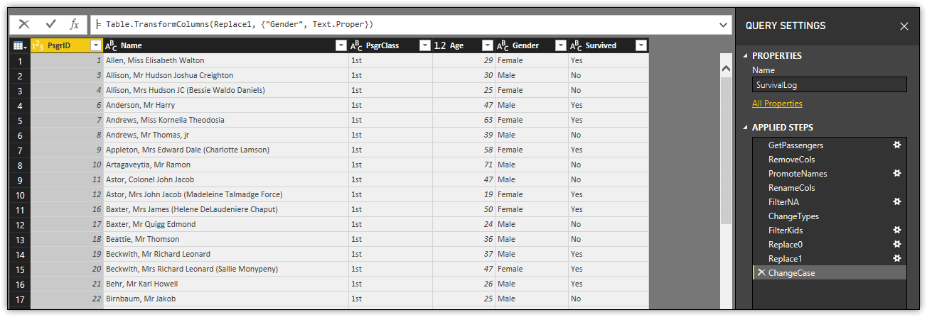
Notice that the Applied Steps section includes one step for each variable defined in the let statement, specified in the same order they appear in the statement. If you select a step, the data displayed in the main windows will reflect the contents of the related variable.
Adding a Calculated Column to a Dataset
Up to this point, each procedural step in your let statement represents a discrete action that is built on the preceding step. In some cases, however, you might need to structure your steps in a way that is not quite so linear. For example, you might want to create a calculated column that shows the difference between a passenger’s age and the average age for that person’s gender. The following steps outline one approach you can take to this column:
- Calculate the average age of the female passengers and save it to a variable.
- Calculate the average age of the male passengers and save it to a variable.
- Add a column that uses the two variables to calculate the age differences.
- Round the age differences to a more readable number of decimals. (This step is optional.)
To carry out these steps, add the following procedural steps to your let statement:
|
1 2 3 4 5 6 |
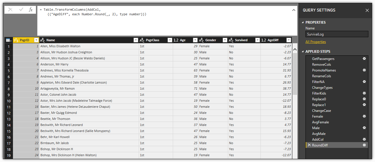
// add calculated column based on average ages Female = Table.SelectRows(ChangeCase, each [Gender] = "Female"), AvgFemale = List.Average(Table.Column(Female, "Age")), Male = Table.SelectRows(ChangeCase, each [Gender] = "Male"), AvgMale = List.Average(Table.Column(Male, "Age")), AddCol = Table.AddColumn(ChangeCase, "AgeDiff", each if [Gender] = "Female" then [Age] - AvgFemale else [Age] - AvgMale),RoundDiff = Table.TransformColumns(AddCol, {"AgeDiff", each Number.Round(_, 2)}) |
I’ll walk you through these steps in smaller chunks so you can better understand how they work. The first line, which is preceded by two forward slashes, indicates a single-line comment. Anything after the slashes to the end of the line is informational only and does not get processed. Power Query also supports multi-line comments that begin with /* and end with */, just like multi-line comments in SQL Server.
It’s up to you whether you want to include comments. Whether or not you do, the next step is to calculate the average age of the female passengers. The following two procedural steps give you the value of the age of the average female.
|
1 2 |
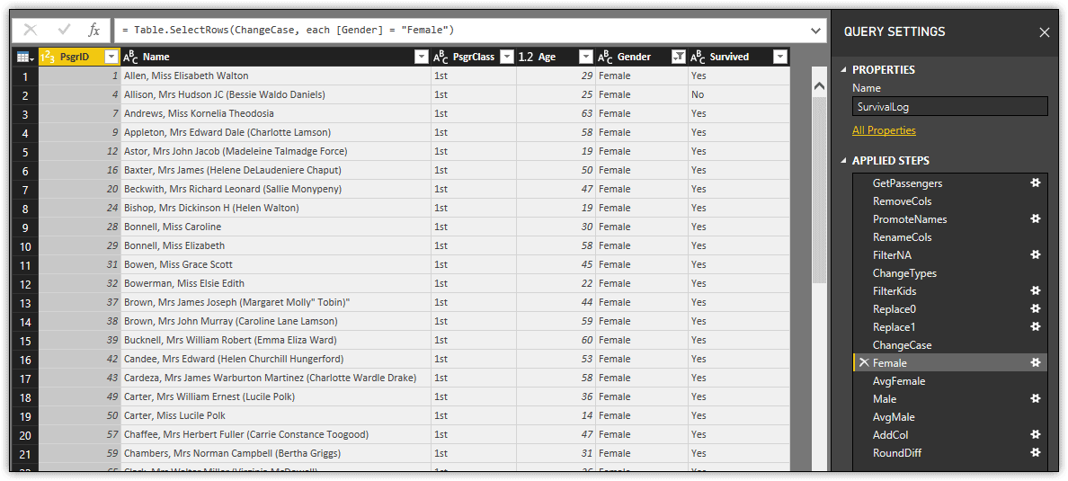
Female = Table.SelectRows(ChangeCase, each [Gender] = "Female"), AvgFemale = List.Average(Table.Column(Female, "Age")), |
The first step uses the Table.SelectRows function to generate a table that includes only rows with a Gender value of Female. The function is being used here in the same way you saw earlier, except that different data is being filtered out and the results are being saved to the Female variable. Notice that the source table for the function is the ChangeCase variable from the preceding step.
The second step uses the List.Average function to calculate that average for the Age values in the Female table. The expression returns a scalar value, which is saved to the AvgFemale variable. The function requires only one parameter. The parameter includes a second function, Table.Column, which passes the values from the Age column to the List.Average function.
The next step is to find the average age of the male passengers. For this, you can use the same construction, with a few minor changes:
|
1 2 |
Male = Table.SelectRows(ChangeCase, each [Gender] = "Male"), AvgMale = List.Average(Table.Column(Male, "Age")), |
Notice that you must again use the ChangeCase variable for the source table when calling the Table.SelectRows function, even though it is no longer the step directly preceding the new one. You can, in fact, use any of the previous variables in your expressions, as long as it makes sense to do so.
With the AvgFemale and AvgMale variables in place, you can now add the column, using the Table.AddColumn function:
|
1 |
AddCol = Table.AddColumn(ChangeCase, "AgeDiff", each if [Gender] = "Female" then [Age] - AvgFemale else [Age] - AvgMale), |
The Table.AddColumn function requires three parameters. The first is the target table, which is again ChangeCase, and the second is the name of the new column, AgeDiff.
The third argument is the expression used to generate the column’s values. The expression starts with the each keyword, which iterates through each row in the target table. This is followed by an if…then…else expression that calculates the row’s value based on whether the passenger is male or female. If the Gender value equals Female, then the AgeDiff value is set to the Age value minus the AvgFemale value, otherwise set the AgeDiff value is set to the Age value minus the AvgMale value.
After defining the new column, the final procedural step rounds the AgeDiff values to two decimal points:
|
1 |
RoundDiff = Table.TransformColumns(AddCol, {"AgeDiff", each Number.Round(_, 2)}) |
The expression includes the Table.TransformColumns function, which you saw earlier, but uses the Number.Round function to round the values, rather than changing their case. The Number.Round function takes two parameters. The first value is an underscore, which represents the column’s current value. The second value, 2, indicates that the value should be rounded to two decimal places.
That completes the steps necessary to create the calculated column. Your let expression, in its entirety, should now look like the following code:
|
1 2 3 4 5 6 7 8 9 10 11 12 13 14 15 16 17 18 19 20 21 22 |
let GetPassengers = Csv.Document(File.Contents("C:\DataFiles\titanic.csv"), [Delimiter=",", Encoding=1252]), RemoveCols = Table.RemoveColumns(GetPassengers, "Column7"), PromoteNames = Table.PromoteHeaders(RemoveCols, [PromoteAllScalars=true]), RenameCols = Table.RenameColumns(PromoteNames, {{"", "PsgrID"}, {"PClass", "PsgrClass"}, {"Sex", "Gender"}}), FilterNA = Table.SelectRows(RenameCols, each [Age] <> "NA"), ChangeTypes = Table.TransformColumnTypes(FilterNA, {{"PsgrID", Int64.Type}, {"Age", Number.Type}}), FilterKids = Table.SelectRows(ChangeTypes, each [Age] > 5), Replace0 = Table.ReplaceValue(FilterKids, "0", "No", Replacer.ReplaceText, {"Survived"}), Replace1 = Table.ReplaceValue(Replace0, "1", "Yes", Replacer.ReplaceText, {"Survived"}), ChangeCase = Table.TransformColumns(Replace1, {"Gender", Text.Proper}), // add calculated column based on average ages Female = Table.SelectRows(ChangeCase, each [Gender] = "Female"), AvgFemale = List.Average(Table.Column(Female, "Age")), Male = Table.SelectRows(ChangeCase, each [Gender] = "Male"), AvgMale = List.Average(Table.Column(Male, "Age")), AddCol = Table.AddColumn(ChangeCase, "AgeDiff", each if [Gender] = "Female" then [Age] - AvgFemale else [Age] - AvgMale), RoundDiff = Table.TransformColumns(AddCol, {"AgeDiff", each Number.Round(_, 2)})in RoundDiff |
The following figure shows what your dataset should now look like in Query Editor.
Notice that the Applied Steps section includes the variables used to find the average ages, even though the AddCol step in the code builds on the ChangeCase variable. You can view the contents of these variables by selecting the step in the Applied Steps section. For example, the following figure shows the data saved to the Female variable.
If you select one of the variables used to store the actual average, Query Editor will display only its scalar value, as shown in the following figure.
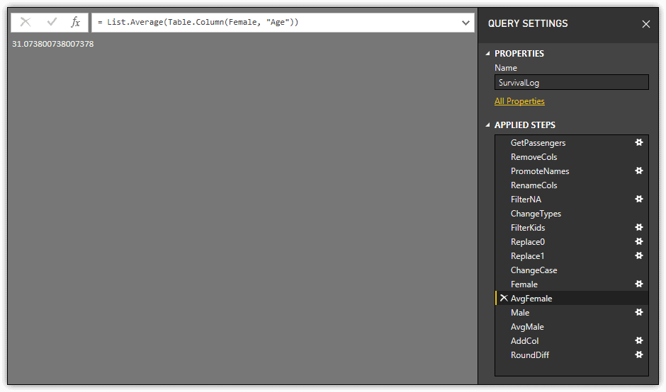
Now Query Editor shows only the contents of the AvgFemale variable, a rather lengthy number. You can see why I included the final procedural step to round the values in the calculated column.
Navigating the Power Query M Formula Language
Not surprisingly, there’s much more to Power Query that what was covered here, but this should give you the foundation you need to start building your own queries in Power BI Desktop. It should also give you a better understanding of how queries are constructed when using point-and-click features to import and transform your data. In this way, you can examine the code to better to understand why you might not be getting the results you expect. You can also start building your query by using point-and-click operations and then use the Advanced Editor to fine-tune your datasets or introduce logic not easily achieved through the interface.
To make the most of Power Query in Power BI Desktop, you’ll need to dig a lot deeper into the language’s various elements than what we’ve covered here, especially the built-in functions. Keep in mind, though, that Power Query was built with Excel in mind, so you might run into elements that don’t transfer easily to the Power BI Desktop environment. Even so, the basic principles that define the language and its syntax are the same, and the better you understand them, the more powerful a tool you have for working with data in Power BI Desktop.
You may also be interested in:
Visualizing SQL Server Audit data in Power BI with tables and charts
FAQs: Power BI Introduction: Power Query M Formula Language in Power BI Desktop — Part 6
1. What is the Power Query M language in Power BI?
Power Query M (also called the M formula language or M language) is the functional programming language that Power BI Desktop uses to define data transformation queries. Every transformation you apply in the Power Query Editor UI generates M code in a let…in expression. The let block defines a series of named steps (Step1 = expression, Step2 = transform(Step1), …) and the in clause specifies the final result. You can view and edit the M code directly in the Advanced Editor. M is case-sensitive and functional – each step is a pure function applied to the previous result.
2. How do I view and edit Power Query M code in Power BI?
In Power BI Desktop, open Power Query Editor (Home > Transform Data). Select a query in the left panel. Click View > Advanced Editor to see the complete M code for that query. You can edit the M code directly in the Advanced Editor and click Done to apply changes. Individual step formulas are also visible in the formula bar when you click on a step in the Applied Steps panel. The Power Query M function reference documentation at docs.microsoft.com/en-us/powerquery-m lists all available M functions with examples.
3. What is the difference between Power Query M and DAX in Power BI?
Power Query M and DAX serve different purposes. M runs during data loading and transformation (the ETL stage) – it cleans, reshapes, combines, and filters data before it is loaded into the Power BI data model. DAX runs at report query time – it performs calculations and aggregations on the already-loaded data model, responding to filters and slicers. M changes what data enters the model; DAX changes how the model is analysed. In practice: use M for data cleaning (remove columns, fix types, merge tables); use DAX for analytics (measures, calculated columns, time intelligence).
4. How do I combine data from multiple sources in Power Query M?
Use Table.Combine([Table1, Table2]) to stack tables vertically (same columns). Use Table.NestedJoin or Table.Join to merge tables horizontally (lookup/join on a key column). For CSV files in a folder, use Folder.Contents() to retrieve all files as a binary table, then combine using Table.Combine(List.Transform(…)). In the UI, these operations are the Append Queries (vertical combine) and Merge Queries (horizontal join) commands under the Home tab in Power Query Editor.
This document contains proprietary information and is protected by copyright law.
Copyright © 2026 Red Gate Software Limited. All rights reserved


Load comments