
In this article I will describe a way to couple SQL Server together with R, and show how we can get a good set of data mining possibilities out of this fusion. First I will introduce R as a statistical / analytical language, then I will show how to get data from and to SQL Server, and lastly I will give a simple example of a data analysis with R.
What is R and what noticeable features does it have
R is an open source software environment which is used for statistical data analysis. All operations are performed in memory, which means that it is very fast and flexible as long as there is enough memory available.
R does not have a storage engine of its own other than the file system, however it uses libraries of drivers to get data from, and send data to, different databases.
It is very modular in that there are many libraries which can be downloaded and used for different purposes. Also, there is a rapidly growing community of developers and data scientists which contribute to the library development and to the methods for exploring data and getting value from it.
Another great feature is that it has built-in graphical capabilities. With R it takes couple of lines of code to import data from a data source and only one line of code to display a plot graph of the data distribution. An example of this graphical representation will be given shortly. Of course, aside from the built-in graphics, there are libraries which are more advanced in data presentation (ggplot2, for example) and there are even libraries which enable interactive data exploration.
For more details on R features and on how to install it, refer to the R Basics article, which was recently published on Simple-talk.
Connecting to SQL Server from R
This part assumes that the reader has already gained some familiarity with the R environment and has the R and RStudio installed.
As mentioned, R does not have its own storage engine, but it relies on other systems to store the analyzed data. In this section we will go through some simple examples on how to couple R with SQL Server’s storage engine and thereby read data from, and write data to, SQL Server.
There are several options to connect to SQL Server from R and several libraries we can use: RODBC, RJDBC, rsqlserver for example. For the purpose of this article, however, we will just use the RODBC package
Let’s get busy and setup our R environment.
In order to get the connectivity to SQL Server working, first we need to install the packages for the connection method and then we need to load the libraries.
To install and load the RODBC package, do the following:
- Open the RStudio console (make sure the R version is at least 3.1.3: If it isn’t, then use the updateR() function)
- Run the following command: install.packages(“RODBC”)
- Run the following command: library(RODBC)
Note: the R packages are usually available from the CRAN site, and depending on the server setup, they may not be directly accessible from the R environment, but instead it may be needed to be downloaded manually and installed manually. Here is the link to the package page: RODBC: http://cran.r-project.org/web/packages/RODBC/index.html
Exploring the functions in a package
R provides useful ways of exploring the functions of the R packages, If, for example, we wanted to list all functions in a specific package we would use a function similar to this:
|
1 2 3 4 5 6 7 8 9 |
lsp <- function(package, all.names = FALSE, pattern) { package <- deparse(substitute(package)) ls( pos = paste("package", package, sep = ":"), all.names = all.names, pattern = pattern ) } |
And then we would call it like this:
|
1 |
lsp(RODBC) |
Typing ??RODBC at the command prompt will bring out some help topics about the RODBC package.
Further, typing ? before any of the functions will bring out the help information about a function. For example,
|
1 |
?dbReadTable |
Getting connected
For the purpose of this exercise, we will be using the AdventureWorksDW database (it can be downloaded from here).
Let’s say we are interested in calculating of the correlation coefficient between the annual sales and the actual reseller sales for each reseller. First we will create the following view:
|
1 2 3 4 5 6 7 8 9 10 |
CREATE VIEW [dbo].[vResellerSalesAmountEUR] AS SELECT fact.ResellerKey , SUM(fact.SalesAmount) / 1000 AS SalesAmountK , dimR.AnnualSales / 1000 AS AnnualSalesK FROM [dbo].[FactResellerSales] fact INNER JOIN dbo.[DimReseller] dimR ON fact.ResellerKey = dimR.ResellerKey WHERE fact.CurrencyKey = 36 -- Euro GROUP BY fact.ResellerKey , dimR.AnnualSales |
I have divided the Sales and the Annual Sales amounts by a 1000, so it is easier to work with the numbers later on. We will go in details in the statistical analysis later on; let’s start by getting connected.
First we need to create a variable with our connection string (assuming we have already loaded the library by running library(RODBC) ):
|
1 2 |
cn <- odbcDriverConnect(connection="Driver={SQL Server Native Client 11.0};server=localhost;database=AdventureWorksDW2012;trusted_connection=yes;") |
RODBC connection
And now we can use this variable as a parameter in the different calls to our database. In the RODBC package there are two different ways to connect to the SQL Server: there are two methods sqlFetch and sqlQuery.
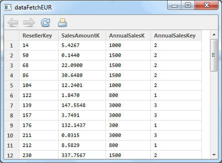
Here is how we use sqlFetch:
|
1 2 |
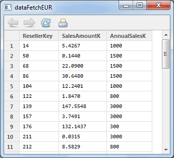
dataFetchEUR <- sqlFetch(cn, 'vResellerSalesAmountEUR', colnames=FALSE, rows_at_time=1000) |
and then we check the contents of the frame with the following command:
|
1 |
View(dataFetchEUR) |
The data looks like this:
Another way to get the data is to use sqlQuery like this:
|
1 |
dataSQLQueryEUR <- sqlQuery(cn, "select * from vResellerSalesAmountEUR") |
As you may have guessed, this is quite flexible if we want to get a subset of the data by using the WHERE clause.
Benchmarking of RODBC
To benchmark the performance of the RODBC library, I have written a script which will read data from SQL Server to R.
Here is the script which will be used:
|
1 2 3 4 5 6 7 8 9 10 11 12 13 14 15 16 17 18 |
library(RODBC) startTime1 <- Sys.time() cn <- odbcDriverConnect(connection="Driver={SQL Server Native Client 11.0};server=localhost;database=TestData;trusted_connection=yes;") readData <- 0 readData <- sqlFetch(cn,'NarrowTable_10k') #readData <- sqlFetch(cn,'NarrowTable_100k') #readData <- sqlFetch(cn,'NarrowTable_1M') #readData <- sqlFetch(cn,'NarrowTable_10M') #readData <- sqlFetch(cn,'NarrowTable_30M') #readData <- sqlFetch(cn,'WideTable_10k') #readData <- sqlFetch(cn,'WideTable_100k') #readData <- sqlFetch(cn,'WideTable_1M') #readData <- sqlFetch(cn,'WideTable_10M') #readData <- sqlFetch(cn,'WideTable_30M') endTime1 <- Sys.time() odbcClose(cn) timeRun <- difftime(endTime1,startTime1,units="secs") print(timeRun) |
The script above creates a connection to a database called TestData. The database has two types of tables – a narrow table with 6 columns and a wide table with 31 columns.
|
1 2 3 4 5 6 7 8 9 10 11 12 13 14 15 16 17 18 19 20 21 22 23 24 25 26 27 28 29 30 31 32 33 34 35 36 37 38 39 40 41 42 43 44 45 46 47 48 49 50 |
CREATE TABLE [dbo].[NarrowTable_X]( [ID] [int] NOT NULL, [Number1] [int] NOT NULL, [Number2] [int] NOT NULL, [Number3] [int] NOT NULL, [Number4] [int] NOT NULL, [Number5] [int] NOT NULL, PRIMARY KEY CLUSTERED ( [ID] ASC )) And CREATE TABLE [dbo].[WideTable_X]( [ID] [int] NOT NULL, [Number1] [int] NOT NULL, [Number2] [int] NOT NULL, [Number3] [int] NOT NULL, [Number4] [int] NOT NULL, [Number5] [int] NOT NULL, [Number6] [int] NOT NULL, [Number7] [int] NOT NULL, [Number8] [int] NOT NULL, [Number9] [int] NOT NULL, [Number10] [int] NOT NULL, [Number11] [int] NOT NULL, [Number12] [int] NOT NULL, [Number13] [int] NOT NULL, [Number14] [int] NOT NULL, [Number15] [int] NOT NULL, [Number16] [int] NOT NULL, [Number17] [int] NOT NULL, [Number18] [int] NOT NULL, [Number19] [int] NOT NULL, [Number20] [int] NOT NULL, [Number21] [int] NOT NULL, [Number22] [int] NOT NULL, [Number23] [int] NOT NULL, [Number24] [int] NOT NULL, [Number25] [int] NOT NULL, [Number26] [int] NOT NULL, [Number27] [int] NOT NULL, [Number28] [int] NOT NULL, [Number29] [int] NOT NULL, [Number30] [int] NOT NULL, PRIMARY KEY CLUSTERED ( [ID] ASC )) |
The X in the table name represents the different amount of data there is in each table. All tables in the database are as follows:
|
1 2 3 4 5 6 7 8 9 10 |
NarrowTable_100k 100k rows NarrowTable_10k 10k rows NarrowTable_10M 10 million rows NarrowTable_1M 1 million rows NarrowTable_30M 30 million rows WideTable_100k 100k rows WideTable_10k 10k rows WideTable_10M 10 million rows WideTable_1M 1 million rows WideTable_30M 30 million rows |
The tables are populated with Redgate’s Data Generator, and then the R script above is used to get all data from the respective table and measure the time it took in seconds.
Here is how long it took (in seconds) to read the 10k, 100k, 1M, 10M and 30M rows:
|
1 2 3 4 5 6 7 8 9 10 11 |
RODBC NarrowTable_100k 0.1120012 NarrowTable_10k 0.05099988 NarrowTable_10M 6.29302 NarrowTable_1M 0.6030009 NarrowTable_30M 17.48804 WideTable_100k 0.322001 WideTable_10k 0.07200003 WideTable_10M 28.01206 WideTable_1M 2.764018 WideTable_30M 80.84013 |
Exploring the data
Now that we have loaded the data into memory, it is time to explore it. First, let’s see the density and the data distribution. R has great facilities to visualize data almost effortlessly. As we will see shortly, we can call a plot a graph with only a few clicks.
First, let’s set the properties of our environment to display two plot graphs in one row. In R this is easily done by using the par() function like this:
|
1 |
par(mfrow=c(1,2)) |
This will create a plot matrix with two columns and one row, which in this case will be filled in by rows. Now, let’s run the two commands which will fill in the graphs in the plot matrix:
|
1 2 |
hist(dataFetchEUR$SalesAmount) hist(dataFetchEUR$AnnualSales) |
This will give us the following graph (found in the Plots section in the RStudio environment):
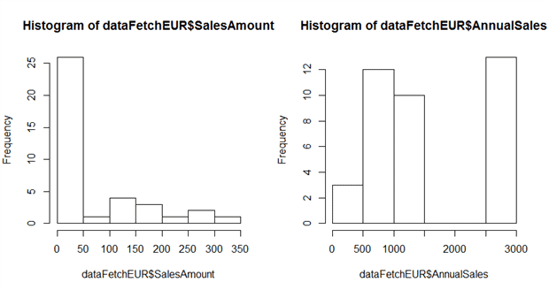
From here we already can extract some valuable knowledge – and we did this with a few clicks! We can see that:
- there are generally two segments of resellers by AnnualSales – ones that peak at around 100K, and the other ones that are above 2.5M
- there are three different segments of resellers by SalesAmount – under 50k, around 150k and around 300k
Remember that this was the data we loaded for the sales in Euros. Let’s load the data from USD sales, and compare the histograms.
We will be using the following view in our database:
|
1 2 3 4 5 6 7 8 9 10 |
CREATE VIEW [dbo].[vResellerSalesAmountUSD] AS SELECT fact.ResellerKey , SUM(fact.SalesAmount) / 1000 AS SalesAmountK , dimR.AnnualSales / 1000 AS AnnualSalesK FROM [dbo].[FactResellerSales] fact INNER JOIN dbo.[DimReseller] dimR ON fact.ResellerKey = dimR.ResellerKey WHERE fact.CurrencyKey = 100 --USD GROUP BY fact.ResellerKey , dimR.AnnualSales |
And then we will use similar commands to load the data in R:
|
1 2 |
dataFetchUSD <- sqlFetch(cn, 'vResellerSalesAmountUSD', colnames=FALSE, rows_at_time=1000) |
And then we get the histograms like this:
|
1 2 |
hist(dataFetchUSD$AnnualSales) hist(dataFetchUSD$SalesAmount) |
The histograms look like this:
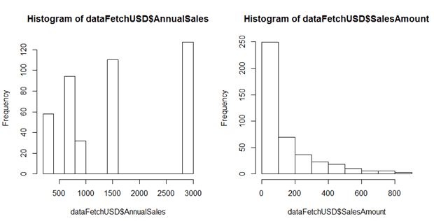
This gives us some more insight into how the resellers perform in the USD market.
Let’s go a bit further ad get a summary of our datasets. Very conveniently there is a built-in function in R, which does exactly that: summarizes our dataset (also called dataframe in R language). If we simply type:
|
1 |
summary(dataFetchEUR) |
We will get the following summary info:
|
1 2 3 4 5 6 7 |
ResellerKey SalesAmountK AnnualSalesK Min. : 14.0 Min. : 0.0315 Min. : 300 1st Qu.:211.2 1st Qu.: 3.4665 1st Qu.: 800 Median :365.0 Median : 12.5177 Median :1500 Mean :373.3 Mean : 65.1193 Mean :1718 3rd Qu.:567.5 3rd Qu.:117.1346 3rd Qu.:3000 Max. :687.0 Max. :337.7567 Max. :3000 |
And respectively for the USD resellers we will type
|
1 |
summary(dataFetchUSD) |
And we will get the summary:
|
1 2 3 4 5 6 7 |
ResellerKey SalesAmountK AnnualSalesK Min. : 1.0 Min. : 0.0013 Min. : 300 1st Qu.:169.0 1st Qu.: 8.8864 1st Qu.: 800 Median :345.0 Median : 54.8905 Median :1500 Mean :348.5 Mean :137.1135 Mean :1593 3rd Qu.:529.0 3rd Qu.:187.1142 3rd Qu.:3000 Max. :700.0 Max. :877.1071 Max. :3000 |
Now let’s do some clustering to dig a bit deeper in our data.
Cluster Analysis
There are countless ways to do Cluster Analysis, and R provides many libraries which do exactly that. There are no best solutions, and it all depends on the purpose of the clustering.
Let’s suppose that we want to help our resellers do better in the Euro region, and we have decided to provide them with different marketing tools for doing that, based on their Annual Sales amount. So for this example, the marketing department needs to have the resellers grouped in three groups based on their AnnualSales and the SalesAmount needs to be displayed for each reseller.
In the example below, we will take the dataFetchEUR dataframe and will divide the resellers in three groups, based on their AnnualSales. Then we will write the data back into our SQL Server Data Warehouse, from where the marketing team will get a report.
By looking at the data summary for the AnnualSales column, we can decide to slice the data by the boundaries of 1,000K and 1,600K. These are imaginary boundaries, which in reality will be set by the data scientist after discussions with the team who will be using the data analysis.
Just to verify, we can group the resellers count per their AnnualSales:
|
1 2 3 4 5 |
SELECT COUNT(*) AS CountResellers , AnnualSalesK FROM [vResellerSalesAmountEUR] GROUP BY AnnualSalesK ORDER BY AnnualSalesK DESC |
We get the following result:
| CountResellers | AnnualSalesK |
| 13 | 3000,00 |
| 10 | 1500,00 |
| 4 | 1000,00 |
| 8 | 800,00 |
| 3 | 300,00 |
So, this seems right. Our three segments will be:
Segment 1 will be < 1,000,000
Segment 2 will be >= 1,000,000 and < 1,600,000
Segment 3 will be > 1,600,000
For this we can use a simple ifelse function to define the clusters:
AnnualSalesHigh.cluster <- ifelse(dataFetchEUR$AnnualSales >= 1600, 3, 0)
AnnualSalesMedium.cluster <- ifelse(dataFetchEUR$AnnualSales >= 1000 & dataFetchEUR$AnnualSales < 1600, 2, 0)
AnnualSalesLow.cluster <- ifelse(dataFetchEUR$AnnualSales < 1000, 1, 0)
Now we have three different datasets, and we need to combine them into one dataset (dataframe). We can use the cbind function like this:
|
1 2 |
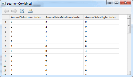
segmentCombined <- cbind(AnnualSalesLow.cluster, AnnualSalesMedium. cluster, AnnualSalesHigh.cluster) |
Now we can look at the segments with the View function:
|
1 |
View(segmentCombined) |
The data looks like this:
Now we need to sum up the values in each row and output another dataframe, which has only one column. We can do this with the following function:
|
1 2 |
AnnualSalesKey <- AnnualSalesHigh.cluster + AnnualSalesMedium.cluster + AnnualSalesLow.cluster |
And finally, we need to bind together the original dataframe and add the categorization per reseller:
|
1 |
dataFetchEUR <- cbind(dataFetchEUR,AnnualSalesKey) |
The data looks like this:
And finally, we will save this dataset into our data warehouse by using the sqlSave function in the RODBC package:
|
1 2 3 |
sqlSave(cn,dataFetchEUR,rownames=FALSE,tablename="Marketing_EURAnnu alSalesCluster",colname=FALSE,append=FALSE) odbcClose(cn) |
And now we have a table called [dbo].[Marketing_EURAnnualSalesCluster] in our [AdventureWorksDW2012] database, which is ready for use by the marketing department.
This process can be automated and a batch file can be created with the R scripts – the entire flow from getting the data to writing it back to the data warehouse – and it can be scheduled to be run regularly.
Conclusion:
In this article we have seen how easy it is to connect to SQL Server from R and do an exploratory data analysis. This brings great value to business, especially because of the time savings of data modelling and visualization techniques which can be very time consuming with other technologies.
We have explored a way to connect to SQL Server (by using the RODBC library) and we have created a simple Cluster Analysis and segmentation, which provides immediate value to the end-users of the data.
Load comments