In this blog, we continue our exploration on PostgreSQL indexes which we started here. In that article, we learned what an index is, and how exactly indexes can help with query execution. But there is much more to learn about indexes! In this blog, we will keep exploring B-tree indexes. We will learn whether (and how) database constraints and indexes are related (or not), how exactly index bitmap scan works, and explore some additional index options available in PostgreSQL.

Indexes and Constraints

In the previous article we learned that the most helpful indexes are indexes with the lowest selectivity, which means that each distinct value in an index corresponds to a small number of rows. The smallest number of rows is one, thereby, the most useful indexes are unique indexes.

The definition of a unique index states just that: an index is unique if for each indexed value there is exactly one matching row in the table. PostgreSQL automatically creates a unique index to support any primary key or unique constraint on a table.

Is there any difference between a primary key and a unique constraint? Many SQL developers assume that a primary key must be an incrementing numeric value and that each table “has” to have a primary key. Although it often helps to have a numeric incremental primary key (which in this case is called a surrogate key), a primary key does not have to be numeric, and moreover, it does not have to be a single-attribute constraint. It is possible to define a primary key as a combination of several attributes; it just has to satisfy two conditions: the combination must be UNIQUE and NOT NULL for all participating attributes. In contrast, UNIQUE constraints in PostgreSQL allow for NULL values.

A table can only have a single primary key (though a primary key is not required), but can also have multiple unique constraints. Any non-null unique set of columns can be chosen to be a primary key for a table; thus, there is no programmatic way to determine the best candidate for a table’s primary key.

Note: If you want to try the code, the appendix has the information you need to install the sample database we will be using, as well as some necessary updates before starting with the current article.

For example, the table booking has a primary key on booking_id and a unique key on booking_ref. Note: you do not need to create a unique constraint to create a unique index:

In this case, both columns are unique, and moreover, there is no need for a booking_id column at all. Booking reference is generated by any reservation system, and it is always both UNIQUE and NOT NULL. The only reason we added a booking_id field to the booking table was to allow application developers to comply to their development standards.

In the case below, the situation is different. The account table has a primary key account_id. When we add a unique index on frequent_flyer_id column, we want to make sure that there will never be two accounts with the same frequent_flyer_id, however, we will have many accounts for which frequent_flyer_id will be null.

What about foreign keys? Do they automatically create any indexes? A common misconception is the belief that the presence of a foreign key necessarily implies the presence of an index on the child table. This is not true.

A foreign key is a referential integrity constraint; it guarantees that for each non-null value in the child table (i.e., the table with the foreign key constraint), there is a matching unique value in the parent table (i.e., the table it is referencing). The column(s) in the parent table must have a primary key or unique constraint on them, however, nothing is automatically created on a child table.

This misconception often backfires when we need to delete a row from a parent table. I observed a user wondering why a deletion of one row (supported by a unique index) took over 10 minutes. It turned out that the table was a parent table for thirteen foreign key constraints, and none of them was supported by an index. To make sure that deletion wouldn’t violate any of these integrity constraints, Postgres had to sequentially scan thirteen large tables.

Does it mean that we always should create an index on column(s) which has a foreign key constraint? Not necessarily. We remember that only indexes with reasonably low selectivity are useful. To illustrate what “reasonable” means in this context, let’s consider the following example.

The flight table in the postgres_air database has a foreign key constraint on the aircraft_code:

This foreign key constraint is necessary because for each flight, there must be a valid aircraft assigned. To support the foreign key constraint, a primary key constraint was added to the aircraft table. That table, however, has only 12 rows. Therefore, it is not necessary to create an index on the aircraft_code column of the flight table. This column has only 12 distinct values, so an index on that column will not be used.

Let’s examine the execution plan for the following query:

The execution plan presented on the Figure 1, and fear not of its size – at this moment, we need just a small portion of it. Pay attention to the lines 19-20:

The PostgreSQL optimizer accesses table statistics and is able to detect that the size of the aircraft table is small and index access won’t be efficient. In contrast, the index on departure_airport field of the flight table proved to be useful due to its low selectivity, and you can see it being used in lines 17-18:

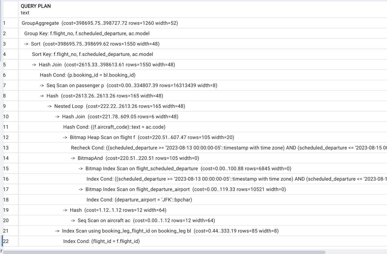
Figure 1. Execution plan with sequential scan on a small table

What does “bitmap” mean?

It has been several times already that the term ‘bitmap’ appeared in execution plans. Each time I promised “to talk about it later,” and now this “later” is here.

It is critically important to fully understand how the indexes bitmapping works in PostgreSQL, especially because other major DBMS do not have similar access methods, documentation does not go into many details about it, and there is a lot of confusion among users regarding how it works. Let’s proceed with uncovering this mystery.

Depending on the index selectivity, PostgreSQL utilizes one of two methods. The first is an index scan; the second depends on a bitmap index scan, followed by a bitmap heap scan.

In the previous blog, we discussed how the index scan works. An index entry includes addresses of the records which match the indexed value; this address contains the block address and the offset of the record within the block. In an index scan, the database engine reads each entry of the index that satisfies the filter condition and retrieves blocks in index order. Because the underlying table is a heap, multiple index entries might point to the same block. If an index has a low selectivity, these situations are rare, and there are high chances that no block will be read (or rather attempted to be read) more than once. However, the situation is different when the selectivity is high, multiple indexes are used, or the filtering condition differs from equal. It these cases, a bitmap index scan will be used. This method builds a heap bitmap in memory. The whole bitmap is a single bit array, with as many bits as there are heap blocks in the table being scanned.

Each index used to satisfy selection criteria is used sequentially. To perform a bitmap index scan, first, a bitmap is created with all entries initially set to 0 (false). Whenever an index entry that matches the search condition is found, the bit corresponding to the heap block indicated by the index entry is set to 1 (true). The second and any additional bitmap index scans do the same thing with the indexes corresponding to the additional search conditions. Once all bitmaps have been created, the engine performs a bitwise logical AND operation to find which blocks contain requested values for all selection criteria, producing a final candidate list. This means that blocks that satisfy only one of the two criteria in a logical AND never have to be accessed. An illustration is shown in Figure 2.

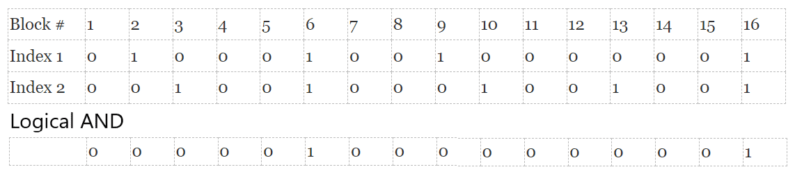
Figure 2. Using bitmaps for table access through multiple indexes

Note, that AND is not the only logical operator which can be used on bitmaps. If some conditions in the selection criteria are connected with OR, the logical OR will be applied, and if a query has more search conditions on a single table, more bitmaps can be put to use.

After the final candidate list is computed, the candidate blocks are read sequentially using a bitmap heap scan (a heap scan based on a bitmap), and for each block, the individual records are examined to re-check the search conditions. Note that requested values may reside in different rows in the same block. The bitmap ensures that relevant rows will not be missed but does not guarantee that all scanned blocks contain a relevant row.

In Figure 1, lines 15 and 17 represent two bitmap index scans, line 14 represents bitmap AND, and line 12 shows bitmap heap scan. To summarize, bitmap access method always includes these three steps:

• Bitmap index scan(s)
• Logical AND/OR
• Bitmap Heap scan

Do we need compound indexes?

Same as other RDBMS, PostgreSQL allows compound (or multi-column) indexes. Since PostgreSQL can utilize multiple indexes for the same query using bitmap index scan, is there any reason to create compound indexes? Let’s run some experiments.

The execution plan for this SELECT statement is presented in Figure 3.

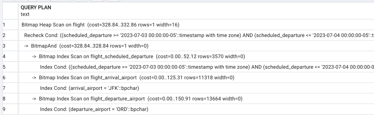
Figure 3. Execution plan with three indexes

There are three indexes which support all three search criteria, and Postgres takes advantage of all three of them. Let’s create a compound index on all three columns:

The new execution plan is presented on Figure 4:

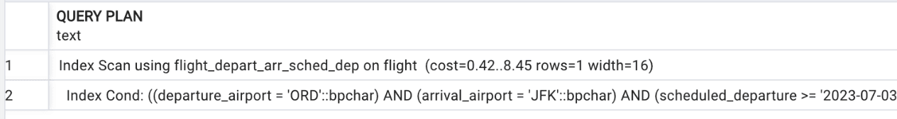
Figure 4. Execution plan with compound index

This new compound index will support searches by departure_airport, by departure_airport and arrival_airport, and by departure_airport, arrival_airport, and scheduled_departure. It will not support, however, the searches by arrival_airport or scheduled_departure. Indeed, recall how b-tree indexes are built and how they are used: we rely on the ordering of indexed values. The values of compound indexes are ordered first by the first column, then be the second column, and so on.

The query

…will produce the execution plan shown in Figure 5.

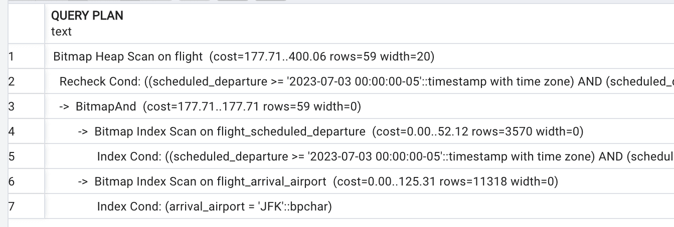
Figure 5. Compound index is not used

On the other hand, the query

…will use the compound index, although only for the first two columns, as shown in Figure 6.

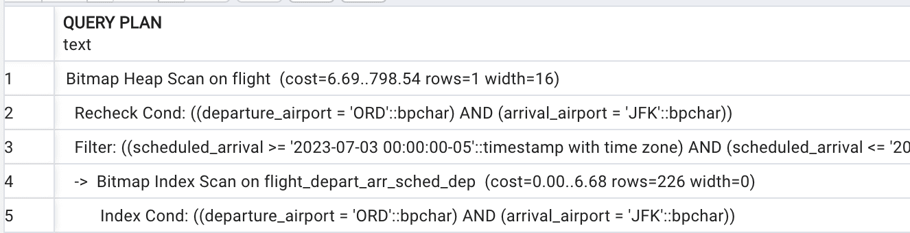
Figure 6. A plan that uses the compound index for the first two columns

In general, an index on (X,Y,Z) will be used for searches on X, (X,Y), and (X,Y,Z) and even (X,Z) but not on Y alone and not on (Y,Z). Thus, when a compound index is created, it’s not enough to decide which columns to include; their order must also be considered.

Why create compound indexes? After all, the previous section demonstrated that using several indexes together will work just fine. Most times, the decision on whether to create a compound index is based on whether they can provide additional selectivity and improve performance of critical queries. I will cover other potential advantages of compound indexes in the next blog.

Summary

PostgreSQL has multiple ways to index the tables, and knowing what available options are can dramatically improve an application performance. Remember, that so far, we only talked about b-tree indexes, and we are not done with them yet, and we didn’t even start talking about other index types!

Did you have fun exploring indexes in PostgreSQL? Would you like to learn more about indexing? Look for the next up in this series.

Appendix – Setting up the training database

If you want to repeat the experiments in this article, the instructions for installing the base database can be found in the Appendix of the first article in this series. If you are starting here, use those instructions to download the database. Once you have downloaded and restored the database, you will need to create the following additional indexes on your copy of the postges_air database:

Don’t forget to run ANALYZE on all the tables for which you build new indexes: