In the previous blog in this series, we learned how to produce, read and interpret execution plans. We learned that an execution plan provides information about access methods, which PostgreSQL use to select records from a database. Specifically, we observed that in some cases PostgreSQL used sequential scan, and in some cases index-based access.

It might seem to be a better idea to talk about indexes before we discussed execution plans, but query plans are a good place to start the performance journey and work our way in! This blog is going to be about indexes, why we need them, how they can help, and how they can make things worse.

What is an index?

What is an index? One might assume that any person who works with databases knows what an index is. However, a surprising number of people, including database developers and report writers and, in some cases, even DBAs, use indexes, even create indexes, with only a vague understanding of what indexes are and how they are structured. Having this in mind, let’s start with defining what is an index.

Since there are many different index types in PostgreSQL (and new index types are constantly created) we won’t focus on structural properties to produce an index definition. Instead, we define an index based on its usage. A data structure is called an index if it is:

• A redundant data structure
• Invisible to an application
• Designed to speed up data selection based on certain criteria

Let’s discuss each of the bullet points in more detail.

Redundancy means that an index can be dropped without any data loss and can be reconstructed from data stored in tables (the postgres_air database dump we will use with the examples comes without indexes, but you can build them after you restore the database. Full instructions are in the appendix of this article to create the database you will need if you wish to follow along with the examples.)

Invisibility means that a user cannot detect if an index is present or absent when writing a query other than the time the query takes to process. That is, any query produces the same results with or without an index.

Finally, an index is created with the hope (or confidence) that it improves performance of a specific query or (even better!) several queries. Although index structures can differ significantly among index types, the speed-up is achieved due to a fast check of some filtering conditions specified in a query. Such filtering conditions specify certain restrictions on table attributes.

Figure 1 shows how an index can speed up the access to the specific table rows.

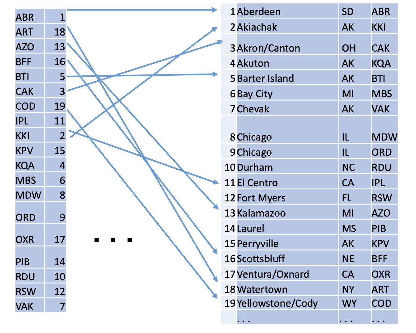
Figure 1. Index access

The right part of Figure 1 shows a table, and the left represents an index that can be viewed as a special kind of a table. Each row of the index consists of an index key and a pointer to a table row. The value of an index key usually is equal to the value of a table attribute. The example in Figure 1 has airport code as its value; hence, this index supports search by airport code.

For this particular index, all values in the airport_code column are unique, so each index entry point to exactly one row in the table. However, some columns, like the column city in the airport table, can have the same value in multiple rows. If this column is indexed, the index must contain pointers to all rows containing this value of an index key. That is, a key may be logically associated with a list of pointers to rows rather than a single pointer.

Figure 1 illustrates how to reach the corresponding table row when an index record is located; however, it does not explain why an index row can be found much faster than a table row. Let’s take a closer look and find out.

Index Types

PostgreSQL supports a lot of types of indexes.

For this article, I am going to only discuss B-Tree indexes because they are the most common index structure you will typically use. There are other types of indexes you can add to tables, but the B-Tree is the most common and what I will focus on for this article. 

The basic structure of a B-tree is shown in Figure 2, using airport codes as the index keys. The tree consists of hierarchically organized nodes that are associated with blocks stored on a disk.

Records in all blocks are ordered, and at least half of the block capacity is used in every block.

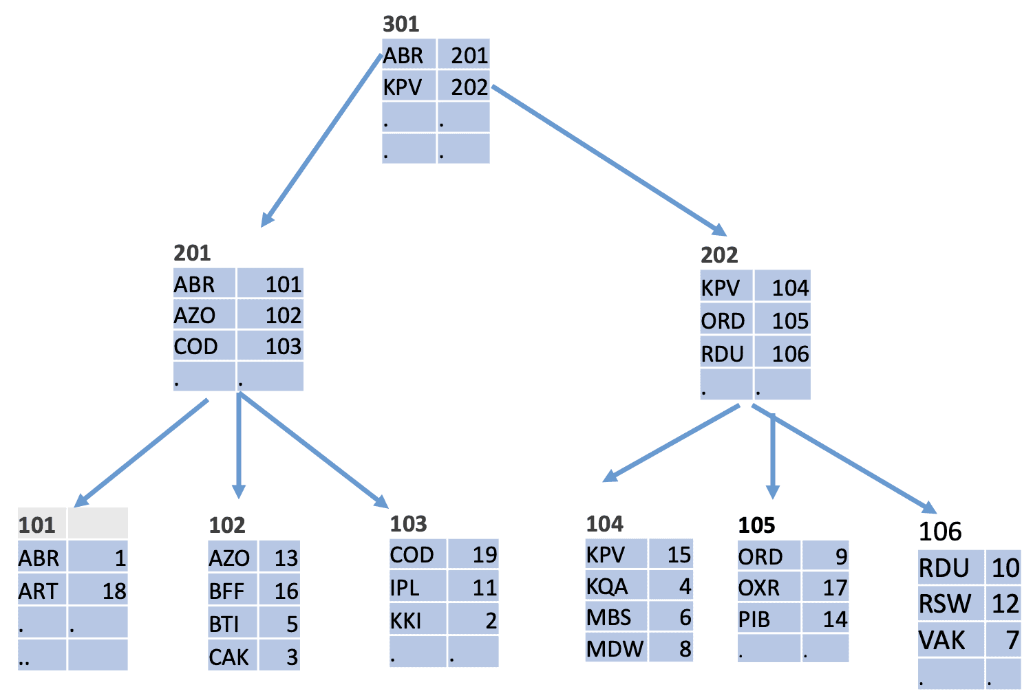
Figure 2. An Example of a B-Tree

The leaf nodes (shown in the bottom row in Figure 2) contain index records exactly like those in Figure 1; these records contain an index key and a pointer to a table row. Non-leaf nodes (located at all levels except the bottom) contain records that consist of the smallest key (in Figure 2, the lowest alphanumeric value) in a block located at the next level and a pointer to this block.

Any search for a key K starts from the root node of the B-tree. During the block lookup, the largest key P not exceeding K is found, and then the search continues in the block pointed to by the pointer associated with P until the leaf node is reached, where a pointer refers to table rows. The number of accessed nodes is equal to the depth of the tree. Of course, the key K is not necessarily stored in the index, but the search finds either the key or the position where it could be located.

B-Tree indexes provide the widest variety of uses (for example, single row and ordered range lookups), and can be built for any data type for which we can define ordering (otherwise called ordinal types), this is where I will start in this series.

When Indexes are Useful

Based on what we learned about indexes so far, would we say that indexes can help to speed up any query? Absolutely not! Whether indexes will be useful or not for a specific query, mostly depends on what type of query we are talking about. It should be no surprise that indexes are most useful for short queries.

But wait – we need to produce one more definition here! Which queries are considered short? Does it depend on the size of a query? The code of the below query is very short; does it mean it’s a short query?

Spoiler alert – it is not! This query produces a Cartesian product of two copies of the airport table, generating a domain of all possible flights.

The next query is “longer”:

However, it is a short query because the result contains just a handful of rows.

Maybe, it’s the number of rows in the output that matters? Wrong again! Look at the next query:

This query produces the output of exactly one row, however, it is a long query because we need to go through all records in flight, booking_leg and passenger tables to obtain the result.

Now, we are ready for a definition:

A query is short when the number of rows needed to compute its output is small, no matter how large the involved tables are. Short queries may read every row from small tables but read only a small percentage of rows from large tables.

How small is a “small percentage”? It depends on system parameters, application specifics, actual table sizes, and possibly other factors. Most of the time, however, it means less than 10%. ratio of rows that are retained to the total rows in the table. This ratio is called selectivity.

Figure 3 presents a graph which shows a dependency between selectivity of the query and a cost of data access with and without indexes.

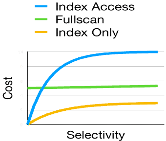
Figure 3. Cost vs Selectivity graph

Note, that PostgreSQL provides two different index-based access methods both of which will be covered in this series of blog posts.

The graph in Figure 3 makes it evident why indexes are most useful for the short queries. For low – selectivity queries, we need to read a small number of rows, thus, the extra cost of additional access to the index pays off. The lower is a query selectivity, the more efficient indexes are. For queries with high selectivity, the cost of additional access to index quickly makes it more expensive than sequential scan.

Execution plans for short queries

When we optimize a short query, we know that in the end, we select a relatively small number of records. This means that the optimization goal is to reduce the size of the result set as early as possible. If the most restrictive selection criterion is applied in the first steps of query execution, further sorting, grouping, and even joins will be less expensive. Looking at the execution plan, there should be no table scans of large tables. For small tables, a full scan may still work.

You can’t select a subset of records quickly from a table if there is no index supporting the corresponding search. That’s why short queries require indexes on larger tables for faster execution. If there is no index to support a highly restrictive query, one needs to be created. It might seem easy to make sure that the most restrictive selection criteria are applied first; however, this isn’t always straightforward.

Let’s look at the following query:

Can you tell which selection criteria will be the most restrictive? Not without

Delayed status might be the most restrictive, because ideally, on any given day, there are many more on-time flights than delayed flights.

In our training database, we have a flight schedule for six months, so limiting it by two days might not be very restrictive. On the other hand, usually the flight schedule is posted well in advance, and if we are looking for flights where the timestamp of the last update is relatively close to the scheduled departure, it most likely indicates that these flights were delayed or canceled.

Another factor that may be taken into consideration is the popularity of the airport in question. LAX is a popular airport, and for Listing 5-1, a restriction on update_ts will be more restrictive than on departure_airport.

Let’s look at the execution plan!

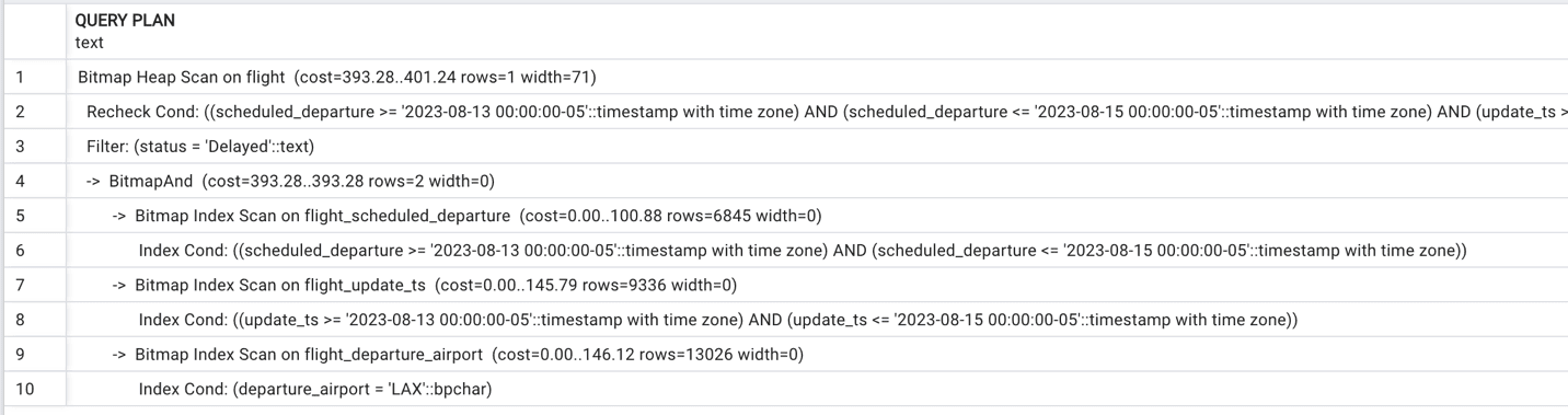
We can see that PostgreSQL query planner took advantage of three indexes on the flight table and performed bitmap index scan – a special kind of index-based data access which I will cover in detail in the next post. In short, the query planner uses three indexes: flight_departure_airport, flight_update_ts and flight_scheduled_departure. Scanning these three indexes helps to identify the blocks which can potentially contain the records which satisfy the search criteria, and then examines these blocks to recheck whether the conditions are indeed met.

What is important for us now is that none of the existing indexes had a clear advantage over others. Does it mean we didn’t build the most restrictive index? Possibly that’s true, we will keep experimenting with additional indexes.

What if we will restrict the time interval even further?

Do you think the execution plan will stay the same or will it change?

Actually, it will!

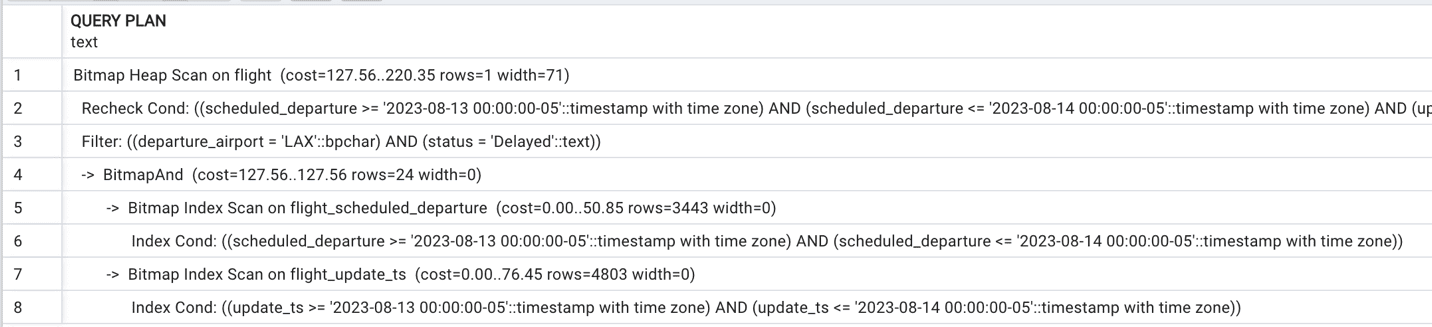
Now, the conditions on both update_ts and scheduled_departure became significantly more restrictive than on departure airport, so only these two indexes will be used.

How about changing the filtering on departure_airport? If we change it to FUK, the airport criterion will be more restrictive than selection based on update_ts and execution plan will change dramatically:

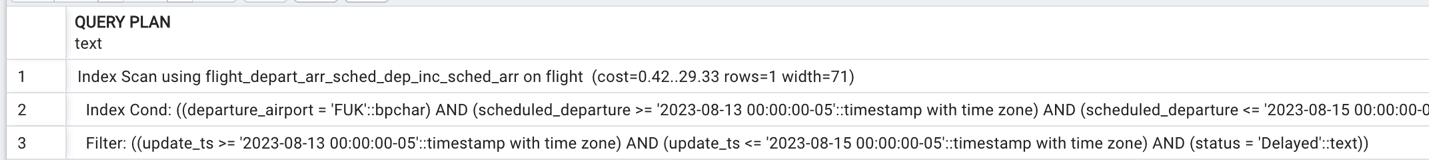
As you can see, if all the search criteria are indexed, there is no cause for concern, PostgreSQL will choose the optimal execution plan. But if the most restrictive criterion is not indexed, the execution plan may be suboptimal, and likely, an additional index is needed.

Performance overhead

The performance improvement does not come for free. As an index is redundant, it must be updated when table data are updated. That produces some overhead for update operations that is sometimes not negligible. However, many database textbooks overestimate this overhead. Modern high-performance DBMSs use algorithms that reduce the cost of index updates, so usually, it is beneficial to create several indexes on a table.

Did you have fun exploring indexes in PostgreSQL? Would you like to learn more about indexing? Look for the next up in this series.

Appendix – Setting up the training database

The instructions for installing the base database can be found in the Appendix of the first article in this series. If you are starting here, use those instructions to download the database.

The experiments in this article require you to create the following additional indexes on your copy of the postges_air database:

Don’t forget to run ANALYZE on all the tables for which you build new indexes: