In the last blog (When PostgreSQL Parameter Tuning is not the Answer), we compared several execution plans for a SQL statement as we made changes to parameters and indexes. Still, there was no mention of what an execution plan is, how one can obtain an execution plan for a query, and how to interpret the result. In this blog, we’ll take a deep dive into this topic.

Why we need an execution plan?

Most likely, if you ever worked with any relational DBMS, you heard the term execution plan, and moreover, you might have seen some of them. But have you ever thought about why you might need an execution plan for a SQL statement? Why you never need to (or get to) produce an execution plan for your C or Java program? The reason is that SQL is a declarative language. That means that when we write a SQL statement, we describe the result we want to get, but we don’t specify how that result should be obtained.

By contrast, in an imperative language (like C), we specify what to do to obtain a desired result—that is, the sequence of steps that should be executed. Sometimes it may not look like it when using modern languages, but once compiled they generally do the steps you program them to.

Note: If you want to execute the samples, in the last section of the article is an appendix with the instructions for preparing the demo.

What is an execution plan?

So, we just sent a SQL statement for PostgreSQL to execute it. Let’s use the same statement we used to illustrate the previous blog:

We sent this to PostgreSQL to execute – what happens next?

To produce query results, PostgreSQL performs the following steps:

• Compile and transform a SQL statement into an expression consisting of high-level logical operations, known as a logical plan.
• Optimize the logical plan and convert it into an execution plan.
• Execute (interpret) the plan and return results.

Compiling a SQL query is similar to compiling code written in an imperative language. The source code is parsed, and an internal representation is generated. However, the compilation of SQL statements has two essential differences.

First, in an imperative language, the definitions of identifiers are usually included in the source code, while definitions of objects referenced in SQL queries are mostly stored in the database. Consequently, the meaning of a query depends on the database structure: different database servers can interpret the same query differently.

Second, the output of an imperative language compiler is usually (almost) executable code, such as byte code for a Java virtual machine. In contrast, the output of a query compiler is an expression consisting of high-level operations that remain declarative—they do not give any instruction on how to obtain the required output. A possible order of operations is specified at this point, but not the manner of executing those operations. The logical plan for the SQL statement presented above is shown below:

Here, project stands for relational operation projection, which reduces the number of columns in the output; filter stands for relational operation filter, which applies selection criteria, join stands for join operation, access identifies that we need to read data from database tables. Note, that the representation above is a “humanized” version of PostgreSQL internal representation of the logical plan, and there is no command that would allow you to actually “see” it.

The instructions on how to execute the query appear at the next phase of query processing, optimization. An optimizer performs two kinds of transformations: it replaces logical operations with their execution algorithms and possibly changes the logical expression structure by changing the order in which logical operations will be executed.

Then, it tries to find a logical plan and physical operations that minimize required resources, including execution time. In this blog, we won’t go into details of how these transformations are done and how the optimizer decides which plan is the best, but we will look at some examples in subsequent blogs. The only thing we need to know now is that the output of the optimizer is an expression containing physical operations. This expression is called a (physical) execution plan. For that reason, the PostgreSQL optimizer is often called the query planner. There are multiple ways you can obtain the physical execution plan for a query, and they will be described later in this blog.

Finally, the query execution plan is interpreted by the query execution engine, frequently referred to as the executor in the PostgreSQL community, and output is returned to the client application.

How is an execution plan built?

The job of the optimizer is to build the best possible physical plan that implements a given logical plan on the server it is executing on. This is a complex process: sometimes, a complex logical operation is replaced with multiple physical operations, or several logical operations are merged into a single physical operation.

To build a plan, the optimizer uses transformation rules, heuristics, and cost-based optimization algorithms. A rule converts a plan into another plan with better cost. For example, filter and project operations reduce the size of the dataset and therefore should be executed as early as possible; a rule might reorder operations so that filter and project operations are executed sooner.

An optimization algorithm chooses the plan with the lowest cost estimate. However, the number of possible plans (called the plan space) for a query containing several operations is huge—far too large for the algorithm to consider every single possible plan, so heuristics are used to reduce the number of plans evaluated by the optimizer.

How to obtain the execution plan?

There are multiple ways to find out the execution plan of any SQL statement, not only SELECT, but also INSERT, UPDATE and DELETE.

The easiest way is to run EXPLAIN command and pass the SQL statement to it:

The result will be a projected execution plan. Remember that in contrast to Oracle or MS SQL Server, PostgreSQL query planner always produces the execution plan right before the execution itself based on many factors, including the current database statistics. (Other RDBMS platforms may reuse previously calculated plans which can have negative, and positive, effects.)

When you execute EXPLAIN PostgreSQL projects the costs of the operations based on the available statistics, which might be not current (or at least, may be in a different state when you actually execute your query to get back data.) Still, running EXPLAIN command would give you a good idea of how your query will be executed.

Another version of the EXPLAIN command is EXPLAIN ANALYZE:

This command produces an execution plan and executes the statement (but does not output the execution results). This allows us to see not only the estimated statistics, but how long the execution took in reality and which original estimates were not right.

Finally, we can run EXPLAIN command with multiple parameters, which are listed below:

• ANALYZE [ Boolean ] – includes actual execution.
• VERBOSE [ Boolean ] – provides more details about plan steps.
• COSTS [ Boolean ] The COSTS parameter defaults to TRUE, including actual when ANALYZE is included– displays projected and actual cost of each plan node (operation in the query).
• SETTINGS [ Boolean ] – list of modified configuration parameters.
• BUFFERS [ Boolean ] – Only used when ANALYZE is included, shows the usage of the shared buffers.
• WAL [ Boolean ] – Only used when ANALYZE is included, shows the effect of WAL (Write ahead logging).
• TIMING [ Boolean ] – Only used when ANALYZE is included, – shows execution time for each node of the query plan.
• SUMMARY [ Boolean ] – default TRUE when ANALYZE]- prints the summary
• FORMAT { TEXT | XML | JSON | YAML } – execution plan output format

As an example, you could use the following:

And get the physical execution plan, with verbose details, in an XML format. You can find more information on the SQL Explain page of the PostgreSQL documentation. But EXPLAIN and EXPLAIN ANALYZE will be the two command you will typically use the most.

How to read an execution plan?

Now, let’s finally get back to the execution plans we analyzed in the previous blog. These execution plans were produced using command EXPLAIN (ANALYSE, BUFFERS, TIMING). Since in this blog, we are focusing on understanding the execution plan itself, we will produce a more compact version of that plan, using EXPLAIN command with no extra parameters.

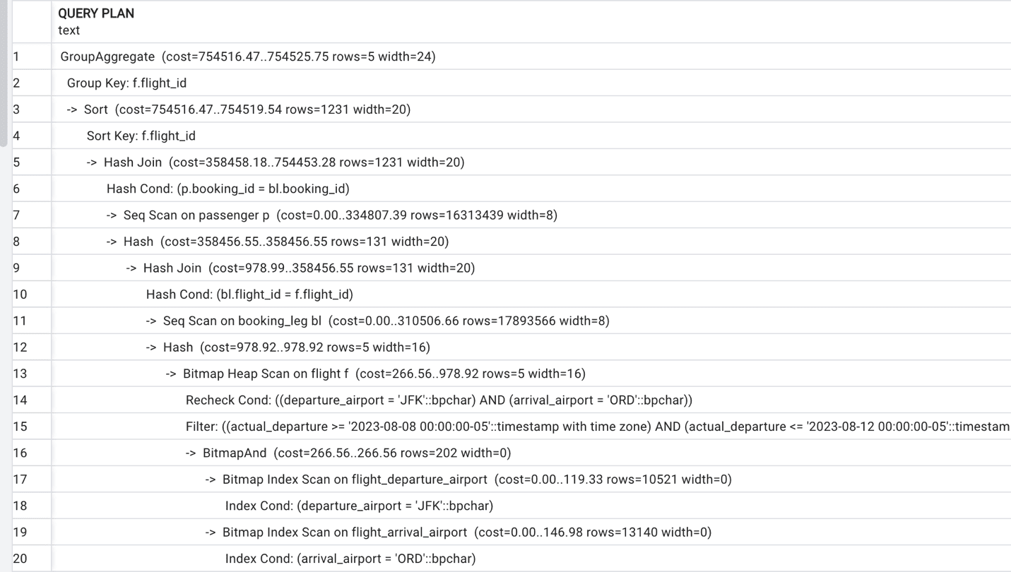Figure 1. The execution plan.

An execution plan is presented as a tree of physical operations. In this tree, nodes represent operations, and arrows point to operands. Looking at Figure 1, it might be not quite clear why it represents a tree.

There are multiple tools, including pgAdmin, which can generate a graphical representation of an execution plan. Figure 2 illustrates possible output. A more compact presentation, also produced by pgAdmin, is presented in Figure 3.

(In pgAdmin, the tree output can be obtained in the query editor by clicking on the Explain or Explain Analyze menu icons in the editor. It will output the text of the query plan and the graph. There is also a menu to choose which settings you wish to apply.)

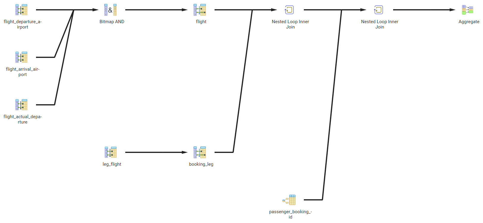
Figure 2.  The Graphical output subtab of Explain

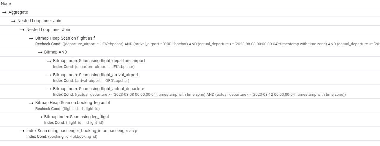
Figure 3.  More compact presentation found in the Analysis subtab of explain.

Now, let’s get back to the actual output of the EXPLAIN command, shown in Figure 1. It shows each node of the tree on a separate line starting with ->, with the depth of the node represented by the offset. Subtrees are placed after their parent node. Some operations are represented with two lines.

The execution of a plan starts from the leaves and ends at the root. This means that the operation that is executed first will be on the line that has the rightmost offset. Of course, a plan may contain several leaf nodes that are executed independently. As soon as an operation produces an output row, this row is pushed to the next operation. Thus, there is no need to store intermediate results between operations.

In Figure 1, execution starts from the last line, accessing the table flight using the index on the departure_airport column. Since several filters are applied to the table and only one of the filtering conditions is supported by the index, PostgreSQL performs a bitmap index scan. The engine accesses the index and compiles the list of blocks that could contain needed records. Then, it reads the actual blocks from the database using bitmap heap scan, and for each record extracted from the database, it rechecks that rows found via the index are current and applies filter operations for additional conditions for which we do not have indexes: arrival_airport and scheduled_departure.

The result is joined with the table booking_leg. PostgreSQL uses a sequential read to access this table and a hash join algorithm on condition bl.flight_id = f.flight_id.

Then, the table passenger is accessed via a sequential scan (since it doesn’t have any indexes), and once again, the hash join algorithm is used on the p.booking_id = bl.booking_id condition.

The last operation to be executed is grouping and calculating the aggregate function sum(). Sorting would produce the list of all flights which satisfy selection criteria (there will be four of them). Then, the count of all passengers on each flight is performed.

Understanding Execution Plans

Often, when we explain how to read execution plans in the manner described in the preceding text, our audience feels overwhelmed by the size of the execution plan for a relatively simple query, especially given that a more complex query can produce an execution plan of 100+ lines. Even the plan presented in Figure 1 might require some time to read. Sometimes, even when each and every single line of a plan can be interpreted, the question remains: “I have a query, and it is slow, and you tell me to look at the execution plan, and it is 100+ lines long. What should I do? Where should I start?”

The good news is that most of the time, you do not need to read the whole plan to understand what exactly makes the execution slow. In subsequent blogs we will address different aspects of query optimization and will learn how to interpret execution plans in each case. It may look daunting now, but once you understand a few of the primary operators, it will all start to be clearer.

Appendix – Setting up for the article series

For this series of articles, just like the previous, we will use a database that I have created for performance tuning examples: postgres_air database. If you want to repeat the experiments described in this article, download the latest version of this database (file postges_air_2023.backup) and restore it on a Postgres instance where you are going to run these experiments. We suggest that you do it on your personal device or any other instance where you have complete control of what’s going on, since you will need to restart the instance a couple of times during these experiments. We ran the examples on Postgres version 15.2, however, they will generally work the same at a minimum on versions 13 and 14.

The restore will create a schema postgres_air populated with data but without any indexes except for the ones which support primary/unique constraints. To be able to replicate the examples, you will need to create a couple of additional indexes: