
Jonathan Lewis' continuing series on the Oracle optimizer and how it transforms queries into execution plans:
- Transformations by the Oracle Optimizer
- The effects of NULL with NOT IN on Oracle transformations
- Oracle subquery caching and subquery pushing
- Oracle optimizer removing or coalescing subqueries
- Oracle optimizer Or Expansion Transformations
It’s common knowledge that when you write an SQL statement, you’re describing to the database what you want but not how to get it. It shouldn’t come as a surprise, then, that in all but the simplest cases, the statement that Oracle optimizes isn’t necessarily the statement that you wrote. Putting it another way, Oracle will probably transform your statement into a logically equivalent statement before applying the arithmetic it uses to pick an execution path.
If you want to become skilled in troubleshooting badly performing SQL, it’s important to be able to recognize what transformations have been applied, what transformations haven’t been applied when they could have been, and how to force (or block) the transformations you think will have the greatest impact.
In this article, we’re going to examine one of the oldest and most frequently occurring transformations that the Optimizer considers: unnesting subqueries.
The Optimizer’s wish-list
The “query block” is the starting point for understanding the optimizer’s methods and reading execution plans. Whatever you’ve done in your query, no matter how complex and messy it is, the optimizer would like to transform it into an equivalent query of the form:
|
1 2 3 |
select {list of columns} from {list of “tables”} where list of simple join and filter predicates} |
Optionally your query may have group by, having, and order by clauses as well as any of the various “post-processing” features of newer versions of Oracle, but the core task for the optimizer is to find a path that acquires the raw data in the shortest possible time. The bulk of the optimizer’s processing is focused on “what do you want” (select), “where is it” (from), “how do I connect the pieces” (where). This simple structure is the “query block”, and most of the arithmetic the optimizer does is about calculating the cost of executing each individual query block once.
Some queries, of course, cannot be reduced to such a simple structure – which is why I’ve put “tables” in quote marks and used the word “simple” in the description of predicates. In this context, a “table” could be a “non-mergeable view”, which would be isolated and handled as the result set from a separately optimized query block. If the best that Oracle can do to transform your query still leaves some subqueries in the where clause or select list, then those subqueries would also be isolated and handled as separately optimized query blocks.
When you’re trying to solve a problem with badly performing SQL, it’s extremely useful to identify the individual query blocks from your original query in the final execution plan. Your performance problem may have come from how Oracle has decided to “stitch together” the separate query blocks that it has generated while constructing the final plan.
Case study
Here’s an example of a query that starts life with two query blocks. Note the qb_name() hint that I’ve used to give explicit names to the query blocks; if I hadn’t done this, Oracle would have used the generated names sel$1 and sel$2 for the main and subq query blocks respectively.
|
1 2 3 4 5 6 7 8 9 10 11 |
select /*+ qb_name(main) */ * from t1 where owner = 'OUTLN' and object_name in ( select /*+ qb_name(subq) */ object_name from t2 where object_type = 'TABLE' ) ; |
I’ve created both t1 and t2 using selects on the view all_objects so that the column names (and possible data patterns) look familiar and meaningful, and I’ll be using Oracle 12.2.0.1 to produce execution plans as that’s still very commonly in use and things haven’t changed significantly in versions up to the latest release of 19c.
There are several possible plans for this query, depending on how my CTAS filtered or scaled up the original content of all_objects, what indexes I’ve added, and whether I’ve added or removed any not null declarations. I’ll start with the execution plan I get when I add the hint /*+ no_query_transformation */ to the text:
|
1 2 3 4 5 6 7 8 9 10 11 12 13 |
explain plan for select /*+ qb_name(main) no_query_transformation */ * from t1 where owner = 'sys' and object_name in ( select /*+ qb_name(subq) */ object_name from t2 where object_type = 'TABLE' ) ; select * from table(dbms_xplan.display(format=>'alias -bytes')); |
The plan returned looks like this:
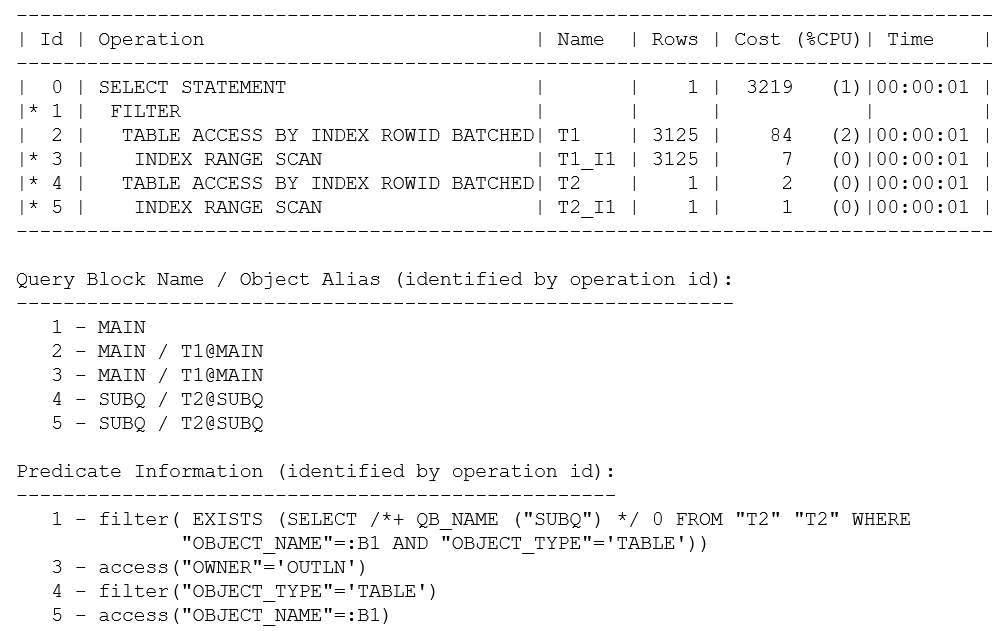
I’ve used explain plan here so that you can see the complete Predicate Information. If I had executed the query and pulled the plan from memory with a call to dbms_xplan.display_cursor(), the predicate information for operation 1 would have read: “1 – filter( IS NOT NULL)”.Since there are no bind variables (and no risk of side-effects due to mismatched character sets), it’s safe to assume that explain plan will produce the correct plan.
There are a few points to pick up on this query and plan:
Even though I have instructed the optimizer to do “no query transformations,” you can see from the Predicate Information for operation 1 that my non-correlated IN subquery has turned into a correlated EXISTS subquery where the correlating object_name has been supplied as a bind variable (:B1). There’s no conflict here between my hint and the optimizer’s transformation – this is an example of a “heuristic” transformation (i.e., the optimizer’s going to do it because there’s a rule to say it can), and the hint relates only to cost-based transformations.
The “alias” information that I requested in my call to dbms_xplan.display() results in the Query Block Name / Object Alias section of the plan being reported. This section allows you to see that the plan is made up of the two query blocks (main and subq) that I had named in the original text. You can also see that t1 and t1_i1 appearing in the body of the plan correspond to the t1 that appeared in the main query block (t1@main), and the t2/t2_i1 corresponds to t2 in the subq query block (t2@subq). This is a trivial observation in this case, but if, for example, you are troubleshooting a long, messy query against Oracle’s General Ledger schema, it’s very helpful to be able to identify where in the query each of the many references to a frequently used GLCC originated.
If you examine the basic shape of this plan, you will see that the main query block has been executed as an index range scan based on the predicate owner = ‘OUTLN’. The subq query block has been executed as an index range scan based on the predicate object_name = {bind variable}. Oracle has then stitched these two query blocks together through a filter operation. For each row returned by the main query block, the filter operation executes the subq query block to see if it can find a matching object_name that is also of type TABLE.
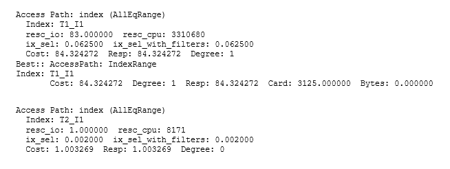
Finally, a comment on Cost: if all you can see is the execution plan, it’s easy to be misled by rounding effects and hidden details of the optimizer allowing for “self-induced caching,” etc. In this case, the base cost of 2 for each execution of the subquery is reduced to 1 in the assumption that the index root block will be cached, and a quick check of the CBO’s trace file (10053 trace) shows that the 1 is actually closer to 1.003 (and the 84 for the t1 access is actually 84.32). Since the optimizer has an estimate of 3,125 rows for the number of rows it will initially fetch from t1 before filtering the total predicted cost of 3219 is approximately: 84.32+ 3125 * 1.003. Realistically, of course, you might expect there to be much more data caching with a hugely reduced I/O load; especially in this case where the total size of the t2 table was only 13 blocks, so a calculation that produced a cost estimate equivalent to more than 3,000 physical read requests for repeated execution of the subquery is clearly inappropriate. Furthermore, the optimizer doesn’t attempt to allow for a feature known as scalar subquery caching so the arithmetic is based on the assumption that the t2 subquery will be executed for each row found in t1.
Here is the section from the CBO’s trace file:
Variations on a theme
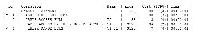
The optimizer transformed an IN subquery to an EXISTS subquery. If the value of the object_name in a row from t1 is of interest if it appears in a list of values, then it’s sensible to check by finding that value in the list. If there are duplicates in the list, stop looking after finding the first match. That’s effectively the method of the FILTER operation in the initial plan, but there is an alternative; if the data sets happen to have the right pattern and volume, Oracle could go through virtually the same motions but use a semi_join, which means “for each row in t1 find the first matching row in t2”. The plan would be like the following:

The semi-join was actually the strategy that the optimizer chose for my original data set when I allowed cost-based transformations to take place, but it used a hash join rather than a nested loop join. Since t2 was the smaller row source, Oracle also “swapped sides” to get to a hash join that was both “semi” and “right”:
But there’s more
The volumes of data involved might mean it’s a good idea to adopt a completely different strategy – and this is where unnesting becomes apparent. If the volume of data from t1 is so small that you only have to run the check a few times, then an existence test could be a very good idea (especially if there’s an index that supports a very efficient check). If the volume of data from t1 is large or there’s no efficient path into the t2 table to do the check, then it might be better to create a list of the distinct values (of object_name) in t2 and use that list to drive a join into t1. Here’s one example of how the plan could change:
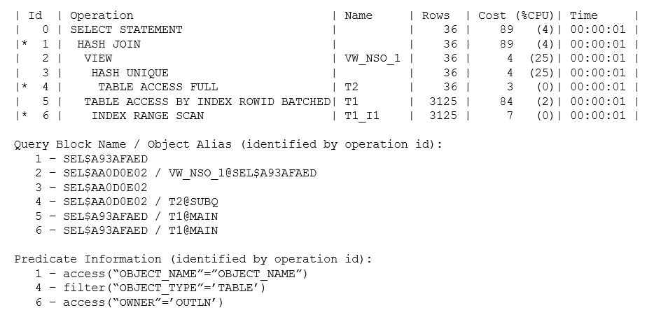
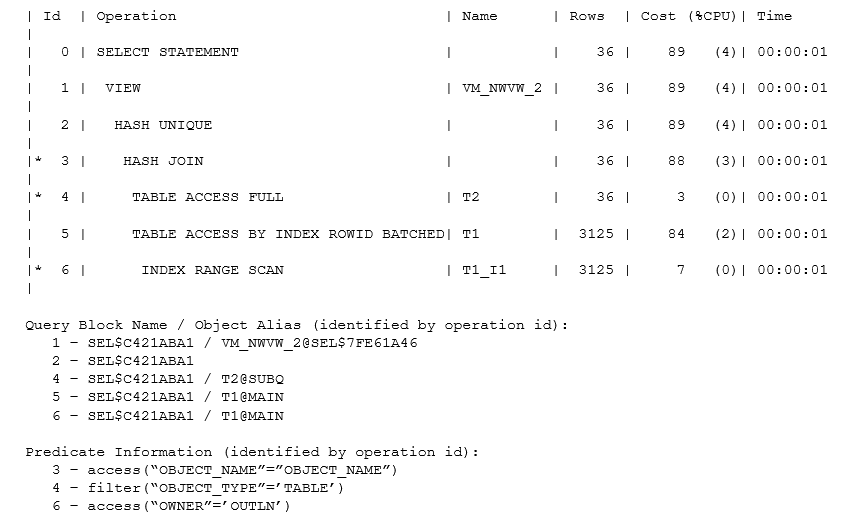
The plan now has a new object at operation 2, a (non-mergeable) view called vw_nso_1 that is recognizably something holding the distinct (hash unique) values of t2.object_name. The number of such values is quite small (only 36 estimated), so the optimizer might have used a nested loop join to collect related rows from t1, but the arithmetic has pushed it into using the “brute force” method of finding all the t1 rows of type TABLE and then doing a hash join.
It’s important to get into the habit of using the alias format option when the shape of the plan doesn’t match the pattern you were expecting to see. In this case, you can see from the Query Block Name information that the final plan consists of two new query blocks: sel$aa0d0e02 and sel$a93afaed. The first query block describes how Oracle will produce a “table” representing the list of distinct object names, and the second query block is a simple join of two “tables” with a hash join. Note how the Object Alias information tells you that the view vw_nso_1 originated in the query block sel$a93afaed.
Side Note: A generated query block name is a hash value generated from the names of the query blocks that were used to produce the new query block, and the hashing function is deterministic.
In effect, the original query has been transformed into the equivalent:
|
1 2 3 4 5 6 7 8 9 10 11 12 |
select t1.* from ( select distinct object_name from t2 where object_type=’TABLE’ ) vw_nso_1, t1 where t1.owner=’OUTLN’ and t1.object_name = vw_nso_1.object_name / |
Whenever you see a view in the plan with a name like vw_nso_{number}, it’s an indication that the optimizer has transformed an IN subquery into an inline view in this way. Interestingly, if you manually rewrite a query to change an IN subquery to an EXISTS subquery, you may find that you get precisely the same plan but with a view named vw_sq_{number}.
And even this strategy could be subject to further transformation if the data pattern warranted it. In my test case, the optimizer does a “distinct aggregation” on a number of small rows before joining to another table to produce much longer rows, which means the aggregation step can be quite efficient. But what if there were a large number of rows to aggregate in t2, and what if the rows were close to being unique and were quite long rows – the aggregation step could require a lot of work for very little benefit. If the join to t1 then eliminated a lot of (aggregated) t2 data and the t1 rows in the select list were quite short, it might be more efficient to join t1 and t2 to eliminate lots of long rows before aggregating to eliminate the duplicates, producing a plan like the following:
As you can see, the optimizer has produced a hash join between t1 and t2 before eliminating duplicates with a “hash unique” operation. This is a little more subtle than it looks because if you tried to write a statement to do this, you could easily make an error that eliminated some rows that should have been kept – an error best explained by examining the approximate equivalent of the statement that Oracle has actually optimized:
|
1 2 3 4 5 6 7 8 9 10 11 12 13 14 15 16 17 |
select {list of t1 columns} from ( select distinct t2.object_name t2_object_name, t1.rowid _owed, t1.* from t2, t1 where t1.owner = ‘OUTLN’ and t2.object_name = t1.object_name and t2.object_type = ‘TABLE’ ) vm_nwvw_2 ; |
Notice the appearance of t1.rowid in the inline view; that’s the critical bit that protects Oracle from producing the wrong results. Since the join is on object_name (which is not unique in the view all_objects that I created my tables from), there could be two rows in t1 and two in t2 all holding the same object_name, with the effect that a simple join would produce four rows.
The final result set should hold two rows (corresponding to the initial two rows in t1), but if the optimizer didn’t include the t1 rowid in the select list before using the distinct operator, those four rows would aggregate down to a single row. The optimizer sometimes has to do some very sophisticated (or possibly incomprehensible) work to produce a correctly transformed statement – which is why the documentation sometimes lists restrictions to new transformations: the more subtle bits of code that would guarantee correct results for particular cases don’t always appear in the first release of a new transformation.
You’ll notice that the generated view name, in this case, takes the form vm_nwvw_{number} Most of the generated view names start with vw_ this one may be the one special case. The view shows one of the effects of “Complex View Merging” – hence the vm, perhaps – where Oracle changes “aggregate then join” into “join then aggregate”, which happens quite often as a step following subquery unnesting.
Summary
If you write a query containing subqueries, whether in the select list or (more commonly) in the where clause, the optimizer will often consider unnesting as many subqueries as possible. This generally means restructuring your subquery into an inline view that can go into the from clause and be joined to other tables in the from clause.
The names of such inline views are typically of the form vw_nso_{number} or vw_sq_{number}.
After unnesting a subquery, Oracle may apply further transformations that make the inline view “disappear” – turning into a join, or semi-join, or (an example we have not examined) an anti-join. Alternatively, the inline view may also be subject to complex view merging, which may introduce a new view with a name of the form vm_nwvw_{number} but may result in the complete disappearance of any view operation.
I haven’t covered the topic of how Oracle can handle joins to or from an unnested view if it turns out to be non-mergeable, and I haven’t said anything about the difference between IN and NOT IN subqueries. These are topics for another article.
Finally, I opened the article with a discussion of the “query block” and its importance to the optimizer. Whenever you write a query, it is a good idea to give every query block its own query block name using the qb_name() hint. When you need to examine an execution plan, it is then a good idea to add the alias format option to the call to dbms_xplan so that you can find your original query blocks in the final plan, see which parts of the plan are query blocks create by optimizer transformation, and see the boundaries where the optimizer has “stitched together” separate query blocks.
Footnote
If you’ve been examining these execution plans in detail, you will have noticed that all five plans look as if they’ve been produced from exactly the same tables – even though my notes were about how different plans for the same query could appear thanks to different patterns in the data. To demonstrate the different plans, I used a minimum number of hints to override the optimizer’s choices. Ultimately, when the optimizer has made a mistake in its choice of transformation, you do need to know how to recognize and control transformations, and you may have to attach hints to your production code.
I’ve often warned people against hinting because of the difficulty of doing it correctly, but hints aimed at query blocks (the level where the transformation choices come into play) are significantly safer than using “micro-management” hints at the object level.
Although I had to use “micro-management” (object-level) hints to switch between the nested loop join and the hash join in the section “Variations on a Theme,” all the other examples made use of query block hints, namely: merge/no_merge, unnest/no_unnest, or semijoin/no_semijoin.
If you liked this article, you might also like Index Costing Threat
This document contains proprietary information and is protected by copyright law.
Copyright © 2026 Red Gate Software Limited. All rights reserved
Load comments