In a recent article on SQL Server Analysis Services 2008, I explained how to implement a multidimensional database. The Analysis Services database I used as an example included a data source, data source view, multiple database dimensions, and a cube based on those dimensions. I then showed you how to deploy the database and browse the cube data in SQL Server Business Intelligence Development Studio (BIDS). However, the cube was missing important functionality-the ability to drill down into the data in order to view aggregated values at more granular levels. That’s because no hierarchies had been created in the database dimensions.

A hierarchy lets you view aggregated fact data at multiple levels. For example, the solution in my recent article contains the Territory dimension, which is based on the DimSalesTerritory table in the Sales data source view (shown in Figure 1).

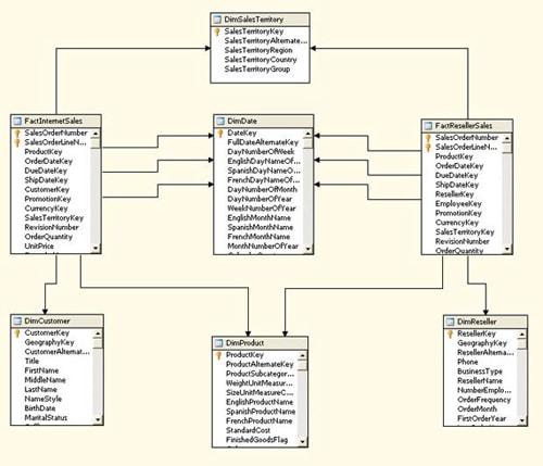
Figure 1: Default diagram from the Sales data source view

The DimSalesTerritory table includes the SalesTerritoryRegion, SalesTerritoryCountry, and SalesTerritoryGroup columns. Although the columns are unrelated in the table, they form a natural hierarchy in which the sales groups contain countries and countries contain regions. If you were to define a hierarchy in the Territory database dimension based on this natural relationship, you could then drill down into the data first by sales group, then by country, and finally by region. And each time you drilled deeper, you would view aggregated data at a more granular level.

In this article, I explain how to implement hierarchies in your Analysis Services database dimensions. The examples in this article are based on the solution in the article mentioned above. For that solution, I created the following database components:

1. A data source that points to the AdventureWorksDW2008 database on a local instance of SQL Server 2008.
2. A data source view that includes the tables shown in Figure 1.
3. Database dimensions for each dimension table in the data source view.
4. A cube based on the database dimensions as well as on the two fact tables in the data source view.

Be sure to refer to the original article for more details about the solution. In addition, if you don’t know how to implement a basic cube in Analysis Services, read that article first and refer to SQL Server Books Online for additional information. Once you know how to implement an Analysis Services database, you’re ready to add hierarchies to your solution.

Creating a Named Query

Before you create any hierarchies in your Analysis Services database, you must ensure that the data supports those hierarchies. For instance, as I mentioned above, the data already supports a hierarchy based on the sales territory data (sales group, country, and region).

However, you might want to implement a hierarchy that the data does not support. For example, suppose you want to create a hierarchy based on the product categories and subcategories. Currently, the DimProduct table in the data source view (shown in Figure 1) includes only the ProductSubcategoryKey column, but no other category-related data. One way to get around this is to replace the DimProduct table with a named query that joins the table to the DimProductSubcategory table and then to the DimProductCateogory table. (You’re essentially flattening out the snowflake configuration of these tables.) A named query is a stored SELECT statement whose results are treated like a table in the data source view.

To replace the DimProduct table with a named query, open the Analysis Services database solution in BIDS, and then open the Sales data source view. In the default diagram, right-click the DimProduct table, point to Replace Table, and then click With New Named Query. This opens the Create Named Query dialog box (shown in Figure 2).

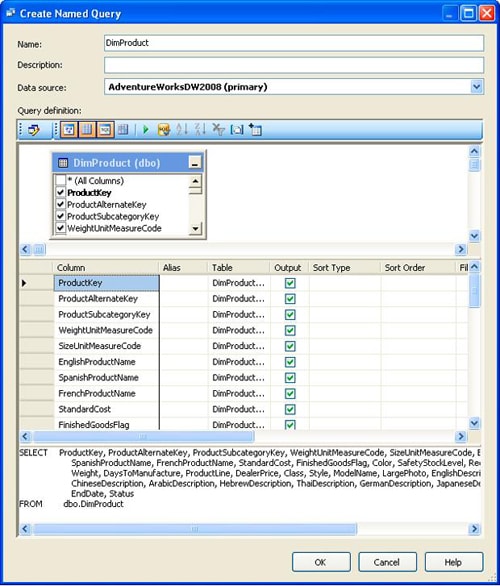
Figure 2: Default view in the Create Named Query dialog box

As Figure 2 shows, when you open the dialog box to replace a table, the dialog box includes details about the table in the three panes: Diagram, Grid, and SQL. You can create your named query by adding the DimProductSubcategory and DimProductCategory tables and then selecting the columns you want to include, or you can simply write the SELECT statement. For this example, I wrote the following statement:

There are a few items in this statement you should note. First, I include only those columns I know I need in my dimensions. Normally, when you add a table to a data source view without modifying the SELECT statement, all columns are included, as was the case with the original solution. Because I don’t need all columns, I bring in only the ones I’m going to use now. However, you can modify a data source view at any time. Just be aware of how your modifications affect the dimensions and cubes that rely on the data source view.

Another component of the SELECT statement worth noting is that I use inner joins to join the tables. I did this because I want to include only those products that are associated with subcategories and categories. I also limit the results to those products that include a list price. That way, only products that are for sale are included in the cube data.

Finally, I use CASE statements in the SELECT statement to handle those products for which there are no French or Spanish names. Because the source columns for the data are not null, missing product names are treated as empty strings. Attribute relationships, which I describe later, do not like empty strings or nulls, so better to sidestep this problem now.

After you create the SELECT statement, you can test whether it’s returning the results you want by clicking the Run button. The results are displayed in the Result pane, shown in Figure 3. (The Diagram pane and Grid pane have been closed.) If you’re satisfied with the results, click OK to close the Create Named Query dialog box. Your data source view should now include the modified table.

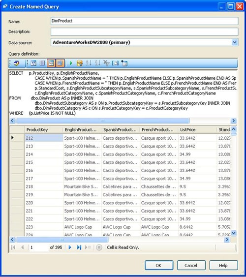
Figure 3: Running a query in the Create Named Query dialog box

That’s all there is to creating a named query. You can now use it as you would any other table. In addition, now that you’ve included the category information, you can create a hierarchy that lets you drill down into the data.

Creating a User-Defined Hierarchy

You create hierarchies in the database dimensions that are used by the cubes. However, you must first ensure that any changes you made to the data source view are reflected in the dimensions. In this case, you’ll need to add the category-related attributes to the Product database dimension, as shown in Figure 4.

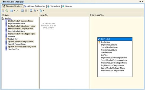
Figure 4: Adding attributes to the Product dimension

To add the category-related attributes to the Product dimension, open the dimension in BIDS and drag the following columns from the DimProduct table (in the Data Source View pane) to the list of attributes (in the Attributes pane):

• EnglishProductSubcategoryName
• SpanishProductSubcategoryName
• FrenchProductSubcategoryName
• EnglishProductCategoryName
• SpanishProductCategoryName
• FrenchProductCategoryName

After you add the attributes, you’re ready to create the hierarchies. You’ll be creating three hierarchies, one for each language. For example, the English hierarchy will include the English Product Category Name attribute (top level), English Product Subcategory Name attribute (middle level), and English Product Name attribute (bottom level).

To create a hierarchy, drag the attribute that represents the highest level of the hierarchy to the Hierarchy pane. For the first hierarchy, start with the English Product Category Name attribute. When you drag the attribute to the Hierarchies pane, the hierarchy is automatically created, as shown in Figure 5.

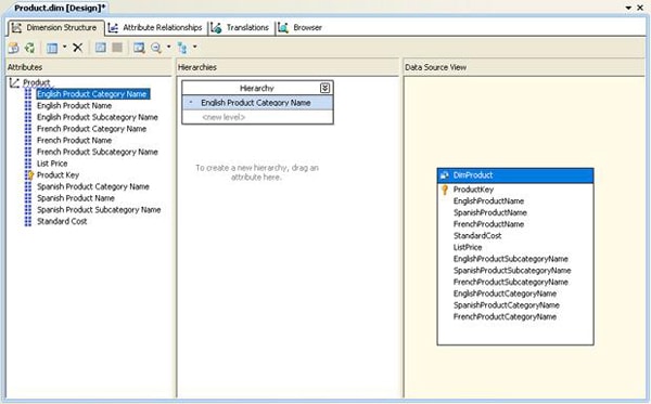
Figure 5: Adding a user-defined hierarchy to the Product dimension

Notice in Figure 5 that, after you add the first level of a hierarchy to create a new hierarchy, you’ll see a blue squiggly line beneath the name of the dimension in the Attributes pane. The line shows that there is a warning about the hierarchy. The warning states that you should avoid visible attribute hierarchies if those attributes are used in the user-defined hierarchies. In other words, if you’re going to include an attribute in a user-defined hierarchy, make it invisible in the attribute tree so users can’t see it when they browse cube data. That way, users will see only the attributes from the user-defined hierarchy. (Some prefer to keep the attributes visible in the tree.) If you decide to hide the attributes, which I’ve done for this solution, set the value of the AttributeHierarchyVisible property to False for each attribute in a user-defined hierarchy. The warning message will go away.

To add the next level of the hierarchy-English Product Subcategory Name-drag the attribute to the Hierarchies pane and drop it into the hierarchy box, where it says <new level>. Then do the same for the English Product Name attribute. After you’ve added the third level of the hierarchy, your Hierarchy pane should look similar to Figure 6.

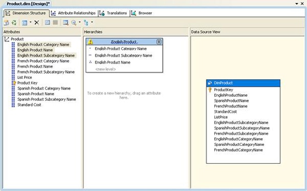
Figure 6: Adding a user-defined hierarchy to the Product dimension

After you’ve created the hierarchy, you can modify its properties. For example, as you can see in Figure 6, I changed the value of the Name property to English Product. Notice, however, that the hierarchy includes a warning message. This one is telling you that attribute relationships have not been defined between levels of the hierarchies, so let’s look at how to do that.

Creating an Attribute Relationship

Attribute relationships improve the performance of Analysis Services when aggregating data. When an attribute relationship is defined between levels of a hierarchy, the engine can use the aggregations of one level to calculate the aggregations of another level, which is why you always receive a message that warns you to create those relationships.

To define an attribute relationship on the English Product hierarchy, select the Attribute Relationships tab for the Product dimension (shown in Figure 7). The tab shows a graphical representation of the default relationships as they apply to your user-defined hierarchies. In addition, the tab includes the Attributes pane, which lists all the dimension’s attributes, and the Attribute Relationships pane, which lists all the dimension’s default relationships-those that exist between the attribute key and each of the other attributes.

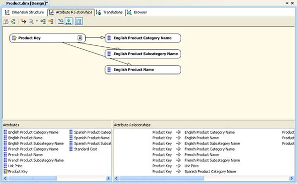
Figure 7: Default attribute relationships for the Product dimension

Notice in Figure 7 that a relationship exists between the Product Key attribute and each of the three attributes in the hierarchy. However, to improve performance, the relationships should be defined between the following pairs of attributes:

• Product Key and English Product Name
• English Product Name and English Product Subcategory Name
• English Product Subcategory Name and English Product Category Name

As you can see, the relationships follow the steps of the hierarchy. You can easily create these relationships in the graphical portion of the Attribute Relationships tab. First, drag the English Product Name attribute to the English Product Subcategory Name attribute. (You always drag from the lower level of the hierarchy to the next level up.) Then drag the English Product Subcategory Name attribute to the English Product Category Name attribute. Your Attribute Relationships pane should now look similar to the one shown in Figure 8.

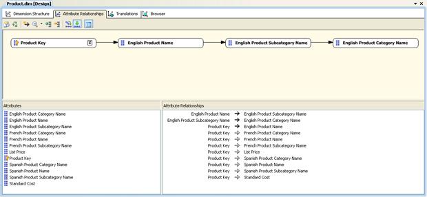
Figure 8: Defining an attribute relationship on the English Product hierarchy

Notice that the Attribute Relationships pane now reflects the new relationships. One other step you can take when defining attribute relationships is to set the relationship type. By default, a relationship is configured as flexible, which means Analysis Services does not retain aggregations when dimensions are updated. However, if you define the relationship as rigid, those aggregations are retained. Although this can improve performance, if a relationship is defined as rigid, Analysis Services will generate an error when processing the dimension, unless it is fully processed. When possible, you should define your attribute relationships as rigid, unless they change frequently. To configure a relationships as rigid, right-click the relationship in the graphical portion of the Attribute Relationships tab, and then select Rigid as the relationship type.

Now you’re ready to create your remaining hierarchies and attribute relationships. (Actually, you could have defined all your hierarchies first and then defined your attribute relationships.)

For this solution, I added hierarchies for the French and Spanish product categories, as shown in Figure 9. When you add the hierarchies, follow the steps you used to create the English Product hierarchy. Also, be sure to rename the hierarchies and, if desired, set the value of the AttributeHierarchyVisible property for each attribute to False.

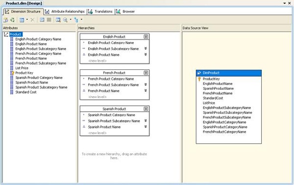
Figure 9: Adding hierarchies for the French and Spanish products

After you’ve added the hierarchies, you can create attribute relationships. Again, follow the steps you followed previously when defining the attribute relationships for the English Product hierarchy. Once you’re completed creating the attribute relationships, your Attribute Relationships tab should look similar to the following:

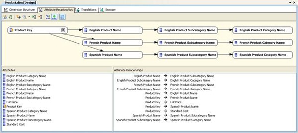
Figure 10: Defining attribute relationships for the French and Spanish products

That’s all there is to creating your hierarchies and attribute relationships. Be sure to save your work and redeploy the database. You’ll then be ready to browse the cube.

Browsing the Cube Data

To browse the cube data in Analysis Services, open the AW_sales cube in BIDS, and then select the Browser tab (shown in Figure 11). Drag the Calendar Year attribute from the Order Date dimension to the Drop Row Fields Here section of the browser, and then drag the Sales Amount measure from the Fact Internet Sales measure group to the Drop Totals or Detail Fields Here section. Now expand the Product dimension in the Measure Group pane. Notice that the hierarchies are included in the dimension tree. Expand the English Product hierarchy, and drag the English Product Category Name attribute to the Drop Column Fields Here section in the browser.

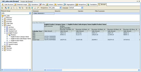
Figure 11: Browsing the cube for products in English

As you can see in Figure 11, I’ve drilled down in the Bikes category and then the Mountain Bikes subcategory. An aggregated value is provided for each product for each year. In addition, if you were to scroll to the right, you would find the total for all mountain bikes for each year, and if you were to scroll all the way to the right, you would find totals for all bikes.

You can just as easily drill down into data for the other languages. For example, Figure 12 shows the aggregated values for products in the Bidon et porte-bidon subcategory of the Accessoire category. Notice that the product Water Bottle is listed in English. That’s because no French name is stored for this product.

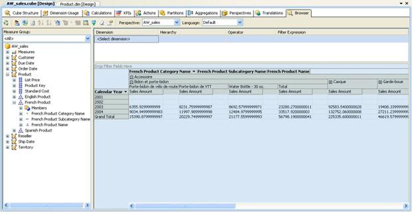
Figure 12: Browsing the cube for products in French

As you can see, the ability to drill into data is a valuable feature when browsing cube data. But you need to implement hierarchies on the database dimensions in order to support that functionality. You can then create the attribute relationships necessary to optimize performance. However, you’re not limited to the hierarchies I’ve described here. For example, you can create a hierarchy based on sales territories, as described earlier in the article. And you can use multiple hierarchies when browsing data. The key is to know the data that you want to include in your cube and to understand the business needs that are driving your decisions for including that data. But as you can see, Analysis Services hierarchies offer plenty of possibilities for displaying that data.