
As part of our continuing series about window functions on SQL Server, we’ll review, in this article, which improvements there are in the next version of SQL Server 2012, and explore how a running aggregation can perform much better by combining the ORDER BY clause with the OVER clause.
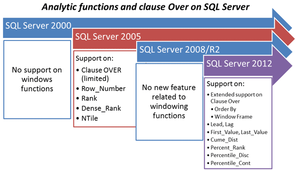
Let’s start with a diagram that shows which of the functions of the SQL ANSI/ISO Standard have been introduced with each of the SQL Server versions:
Along with SQL Server’s growing adoption of the standard, the standard itself has been developing. Here we illustrate the major releases of the Standard of the language SQL adopted by ISO and ANSI.
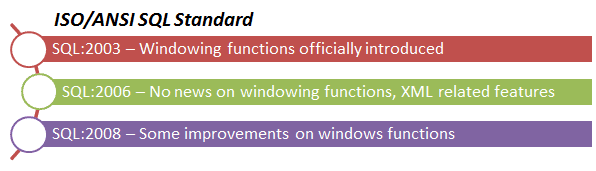
As we know, SQL Server has taken some time to adopt and support all of the windowing functions. The functions we will see in this article were introduced in the ISO/ANSI standard SQL:2008. It has taken four years to implement it in SQL Server, but we are finally getting close to a full support on SQL Server 2012.
Even though we have a very good support for these window functions, I would like to see full support. For instance, as we can see in the pictures, the clause OVER has been supported since SQL Server 2005 but with some limitations; and it was improved on SQL Server 2012, but it still doesn’t yet have full support as you can see in the list of limitations below.
I’ve used the words “getting close” in the sequence above because we still have some unsupported standard functionality. Here is a list of aspects of the standard that are still missing in SQL Server 2012:
- Function FIRST, returns the first value of an ordered group
- MAX(City) KEEP (DENSE_RANK FIRST ORDER BY SUM(Value))*
- Function LAST, returns the last value of an ordered group MIN(City) KEEP (DENSE_RANK LAST ORDER BY SUM(Value))*
- Clause NULLs FIRST and NULLs LAST
- OVER(ORDER BY Coluna1 NULLs FIRST)
- Support on interval frame (Year, Month, Day, Hour, Minute, Second)
- Window Clause
- SELECT LAG(Col1) OVER MyAliasWin AS Col1 FROM Tab1
- WINDOW MyAliasWin AS (ORDER BY Col1 ROWS 2 PRECEDING)
* Not standard (ISO/ANSI) clauses
New functions on SQL Server 2012
I’ll now briefly introduce some important window functions supported on SQL Server 2012. After that I’ll explain how the window frame works so that you can understand better why and when to use it in the clause OVER.
I’ll not cover all the possible syntax options of these functions because these are well covered on Books Online here and here.
If you want to test these functions, you will need the copy of SQL Server 2012 RC0, which you can download here (Editor’s note: this release candidate is no longer available to download from Microsoft).
Here you can see the script to create a table to test the functions:
|
1 2 3 4 5 6 7 8 |
USE TempDB GO IF OBJECT_ID('Tab1') IS NOT NULL DROP TABLE Tab1 GO CREATE TABLE Tab1 (Col1 INT) GO INSERT INTO Tab1 VALUES(5), (5), (3) , (1) GO |
LEAD()
The LEAD function is used to read a value from the next row, or the row below the actual row. If the next row doesn’t exist, then NULL is returned.
|
1 2 3 |
-- LEAD SELECT Col1, LEAD(Col1) OVER(ORDER BY Col1) AS "LEAD()" FROM Tab1 |
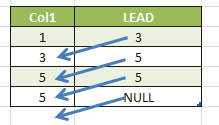
As we can see, the LEAD column has the next row value, but NULL is returned in the last row.
By default, the next row is returned; but you can change this behavior by specifying a parameter to read N following rows, for instance:
|
1 2 3 |
-- LEAD SELECT Col1, LEAD(Col1, 2) OVER(ORDER BY Col1) AS "LEAD()" FROM Tab1 |
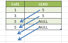
In this last query, I used the parameter “2” in the function in order to specify that I want to read the second row after the current row.
LAG()
The LAG() function is similar to the LEAD() function, but it returns the row before the actual row rather than return the next row. For instance:
|
1 2 3 |
-- LEAD SELECT Col1, LEAD(Col1, 2) OVER(ORDER BY Col1) AS "LEAD()" FROM Tab1 |
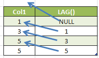
As we can see, the function returns the value of the row before the actual row; but when the row before doesn’t exist, then NULL is returned.
You may be wondering whether I could do the same thing by using the function LEAD() with a negative parameter (OffSet): In other words, instead of read 1 following value I could read -1 following value.
Let’s see a sample:
|
1 2 |
SELECT Col1, LEAD(Col1, -1) OVER(ORDER BY Col1) AS "LEAD() as LAG()" FROM Tab1 |
Msg 8730, Level 16, State 1, Line 1
Offset parameter for Lag and Lead functions cannot be a negative value.
As we can see, we cannot use negative values in this parameter to the function.
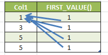
FIRST_VALUE()
As the name says, FIRST_VALUE() returns the first value in a partition window. For instance:
|
1 2 3 |
-- FIRST_VALUE SELECT Col1, FIRST_VALUE(Col1) OVER(ORDER BY Col1) AS "FIRST_VALUE()" FROM Tab1 |
LAST_VALUE()
Also, as the name suggests, it returns the last value in a partition window: For instance:
|
1 2 3 |
-- LAST_VALUE SELECT Col1, LAST_VALUE(Col1) OVER(ORDER BY Col1 ROWS BETWEEN UNBOUNDED PRECEDING AND UNBOUNDED FOLLOWING) AS "LAST_VALUE()" FROM Tab1 |
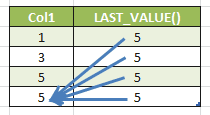
To get the last value in the partition window I’ve specified a different frame. This is what the words “ROWS BETWEEN UNBOUNDED PRECEDING AND UNBOUNDED FOLLOWING” mean. I’ll explain how a window frame works later on this article.
PERCENT_RANK()
In my first article about window functions, I’ve demonstrated the behavior of the RANK() function. The PERCENT_RANK() function is very similar to the RANK() function, but the values that are returned range between 0 and 1.
|
1 2 3 4 |
SELECT Col1, PERCENT_RANK() OVER(ORDER BY Col1) AS "PERCENT_RANK()" RANK() OVER(ORDER BY Col1) AS "RANK()" (SELECT COUNT(*) FROM Tab1) "COUNT" FROM Tab1 |
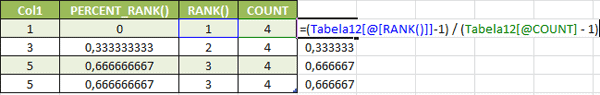
You can do the same thing by calculating the percent rank using the following formula:
- (RANK() – 1) / (NumberOfRows – 1)
CUME_DIST()
The function CUME_DIST() is also used to calculate a rank from 0 to 1 based on the position of the row in the rank, for instance:
|
1 2 3 |
-- CUME_DIST() SELECT Col1, CUME_DIST() OVER(ORDER BY Col1) AS "CUME_DIST()" FROM Tab1 |
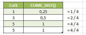
The same behavior could be achieved by using the following formula:
- COUNT(*) OVER (ORDER BY Col1) / COUNT(*) OVER ()
Window Frame
To start investigating, and to understand the concept of a window frame, let’s examine the syntax of a window function and the window frame:
| OVER ( [ <PARTITION BY clause> ] [ <ORDER BY clause> ] [ <ROW or RANGE clause> ] ) |
 |
The window frame is a very important concept when used in windowing and aggregation functions, and it can also be very confusing. One reason for the confusion is that it is also known by the synonymous terms window frame, window size or sliding window. I’m calling this a window frame because this is the term that Microsoft chose to call it in books online.
In the window frame, you can specify the subset of rows in which the windowing function will work. You can specify the top and bottom boundary condition of the sliding window using the window specification clause. The syntax for the window specification clause is:
[ROWS | RANGE] BETWEEN <Start expr> AND <End expr>
Where:
<Start expr> is one of:
- UNBOUNDED PRECEDING: The window starts in the first row of the partition
- CURRENT ROW: The window starts in the current row
- <unsigned integer literal> PRECEDING or FOLLOWING
<End expr> is one of:
- UNBOUNDED FOLLOWING: The window ends in the last row of the partition
- CURRENT ROW: The window ends in the current row
- <unsigned integer literal> PRECEDING or FOLLOWING
Where it is not explicitly specified, the default window frame is “range between unbounded preceding and current row“, in other words, the top row in the window is the first row in the current partition, and the bottom row in the window is the current row.
To see all this theory in practice, let’s consider the following query on the table Orders from the Northwind database:
|
1 2 3 4 5 |
USE NorthWind GO SELECT OrderID, CustomerID FROM Orders WHERE CustomerID IN (1,2) |
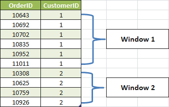
The result of the query returns two customers and their respective orders. In the picture we can see two windows partitioned by CustomerID, where CustomerID = 1 and CustomerID = 2.
Even then, this is not a 100% correct representation of a window, but it’s easier to understand it when we look at the window as it is in the picture; where the windows correspond to each distinct CustomerID.
A more correct picture of a window might be the following:
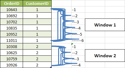
Considering that the first window has 6 rows, we have 6 windows that coexist. Because they coexist, it’s easy to implement the frame in a window. I could tell that a window goes from unbounded preceding to 3 following rows.
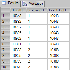
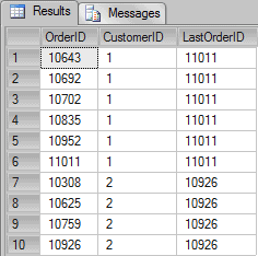
I can understand if this is not quite so straightforward to understand, so let’s, instead, see some examples: Let’s suppose that I want to return the first OrderID of each window above. I could write something like the following query:
|
1 2 3 4 |
SELECT OrderID, CustomerID, FIRST_VALUE(OrderID) OVER(PARTITION BY CustomerID ORDER BY OrderID) AS FirstOrderID FROM Orders WHERE CustomerID IN (1,2) |
Remember, if I don’t specify the window frame clause, then the default is “range between unbounded preceding and current row”. In other words, the query above is equivalent to the following:
|
1 2 3 4 5 6 7 |
SELECT OrderID, CustomerID, FIRST_VALUE(OrderID) OVER(PARTITION BY CustomerID ORDER BY OrderID ROWS BETWEEN UNBOUNDED PRECEDING AND CURRENT ROW) AS FirstOrderID FROM Orders WHERE CustomerID IN (1,2) |
To try to make things clearer, here’s an illustration of the way that the top and bottom boundary works in the query above (using the function FIRST_VALUE). This would work something like this:
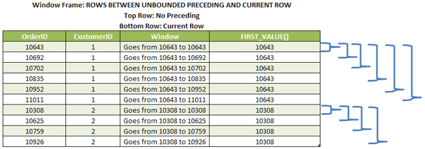
In the picture, we can see that the fist value of the first window is 10643 and the first value of the next window is also 10643, the top row specified in the frame (no preceding) says that it is unbounded preceding.
A good example of how the window frame works is the function LAST_VALUE, because we need to change the default frame in order to really return the last value of a partition.
This function can be a little confusing at first, but as soon we understood the window frame we can see that the action that the function performs by default is correct. It’s very common to test the last_value function and think that this is not working properly, and some people even demand a “fix” for the function because they reckon that it is not working correctly.
Let’s see what the function returns for the same sample in the Orders table:
|
1 2 3 4 5 |
SELECT OrderID, CustomerID, LAST_VALUE(OrderID) OVER(PARTITION BY CustomerID ORDER BY OrderID) AS FirstOrderID FROM Orders WHERE CustomerID IN (1,2) |
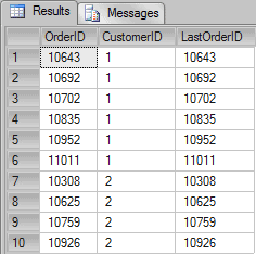
As we can see, the result was not what one might expect. I wanted to return the last OrderID of each customer, and SQL Server is returning the actual (current row ?) OrderID for each row.
Let’s see the same illustration we saw earlier with the first_value function but now using the LAST_VALUE concept:
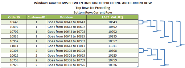
Again, remember that because I didn’t specify the window frame clause in the query, it is using the default frame. If I don’t specify the frame I want, it will use the bottom row as the current row, and it will return the value of the actual row as the last value. If you take a look at the blue brackets, you’ll see that the size of the sliding window is limited to the current row.
Now let’s see the difference when if I specify the frame as unbounded, in the following code:
|
1 2 3 4 5 6 7 |
SELECT OrderID, CustomerID, LAST_VALUE(OrderID) OVER(PARTITION BY CustomerID ORDER BY OrderID ROWS BETWEEN UNBOUNDED PRECEDING AND UNBOUNDED FOLLOWING) AS FirstOrderID FROM Orders WHERE CustomerID IN (1,2) |
Now we’ve got the expected result. Let’s see how the illustration would be for this scenario:
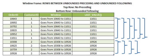
The window frame goes from unbounded preceding to unbounded following. In other words, when SQL Server reads the last value of a window, it goes on until the unbounded following that is the last row in the partition.
RANGE versus ROW
Another confusing thing about the window frame is the RANGE versus ROW. The question is, what is the difference between them?
The ROWS clause limits the rows within a partition by specifying a fixed number of rows preceding or following the current row. Alternatively, the RANGE clause logically limits the rows within a partition by specifying a range of values with respect to the value in the current row. Preceding and following rows are defined based on the ordering specified by the ORDER BY clause. The window frame “RANGE … CURRENT ROW …” includes all rows that have the same values in the ORDER BY expression as the current row.
Again, let’s see this in practice, so as to try to understand it better.
Let’s suppose we have the following query:
|
1 2 3 4 5 6 7 8 9 10 11 12 13 14 15 |
USE tempdb GO IF OBJECT_ID('tempdb.dbo.#TMP') IS NOT NULL DROP TABLE #TMP GO CREATE TABLE #TMP (ID INT, Col1 CHAR(1), Col2 INT) GO INSERT INTO #TMP VALUES(1,'A', 5), (2, 'A', 5), (3, 'B', 5), (4, 'C', 5), (5, 'D', 5) GO --SELECT * FROM #TMP SELECT *, SUM(Col2) OVER(ORDER BY Col1 RANGE UNBOUNDED PRECEDING) "Range" SUM(Col2) OVER(ORDER BY Col1 ROWS UNBOUNDED PRECEDING) "Rows" FROM #TMP |
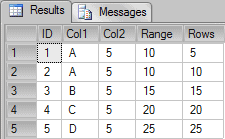
We have two running calculations in this query. One of these is using the RANGE frame and the other is using the ROWS frame. You can see that the result for the value “A” is different for each frame. Let’s try to illustrate these windows:
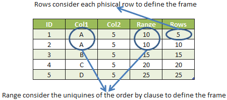
We can see in the picture that the aggregation works differently depending on the frame.
There is another very important difference between the ROW and RANGE clause: the RANGE clause always uses an on-disk window to process the window spool operator. But this is a subject for the next and final article.
Conclusion
Window functions are very powerful, and can help us to think in set based terms, and get more elegant solutions for many problems we have on building efficient T-SQL code for which we’ve formerly required cursors or non-standard SQL.
In the next and final article about window functions I’ll answer the question you may are doing to yourself. What about performance and scalability?
I’ll be describing the window_spool_ondisk_warning eXtended Event, to tell the difference between a on disk window spool versus a on memory window spool. Also we’ll see some performance tests between the actual solutions versus windowing functions. The question is this: Is it really worth changing all my queries to start using windowing functions?
See you soon.
That’s all folks.
This document contains proprietary information and is protected by copyright law.
Copyright © 2026 Red Gate Software Limited. All rights reserved


Load comments