When the user of a database application requests data, or sends a form for processing, they judge the performance of the system on the time they spend waiting and looking at the mouse-pointer in the shape of an hourglass. Often, if this time gets excessive, the database is blamed. The truth is actually more complicated than that.

As a way of illustrating the large number of factors that can affect the responsiveness of an application, we’ll be looking at what happens when that hourglass is showing, and how a problem at almost every stage can affect the performance of the system. This is to show how several important problems can only be detected by inference if progress is monitored only from the perspective of the Database Server, and that a more complete picture can be gained by the addition of an application-based performance profiler.

Here is a graph which gives an overview of the ‘big picture’ of SQL Server incoming requests and outgoing data:

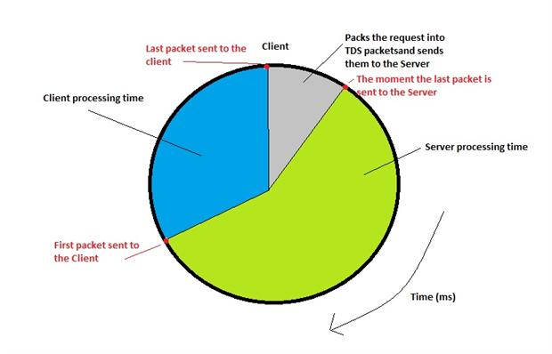
As we can see in the picture above, the lifecycle of a database request starts way before it is processed by the database engine, and it ends much later than the time when the database engine has carried out its tasks.

In other words, there are factors aside from the database engine which affect the hourglass experience.

The urge, however, is often to see the hourglass and assume that ‘the database is running slow’. This insight isn’t going to help to fix the problem. There will be a good reason for that hourglass that won’t go away, and it is very likely to be a specific bug rather than a general malaise. It may even be nothing to do with the database.

And here is the pitfall from the point of view of SQL Server: we cannot see the ‘big picture’ from within SQL Server; i.e. we can only see what waits and performance issues are happening after the last TDS packet has been appended and the processing has started, and we cannot see any performance data after the last TDS packet has left SQL Server on its way to the application.

Let’s look in detail at what exactly happens between the times the hourglass appears to the time when the hourglass disappears, in the context of a single application request.

Network performance issues

All data to and from SQL Server is transferred over the network in the form of TDS (tabular data stream) packets, which are usually 4kb each (it really depends on the environment’s network settings).

After arriving to the doorstep of SQL Server, the incoming TDS packets have to be assembled into their batches before the complete message can be passed to the parser and Query Optimizer (QO).

If a request is sent to SQL Server that is larger than the size of the network packet, then the request will be divided into multiple network packets. This means that there will be some system resources allocated for the assembly of all packets and of course there will be a waiting time until all the packets have arrived.

In the example above we can clearly see that there is a performance degradation related to the use of large requests. In this case, the network adapter was working really hard to receive and queue the network packets. Meanwhile, SQL Server was waiting for all packets belonging to each request and to assemble them, then to parse them, handles the internal work to retrieve the data and eventually to get to the point where it would actually return some data to the application which requested the data a while back.

And of course, whilst we’re on the subject of network traffic, things can go badly wrong in sending data back to the application. Here is another real world example:

You can experience both a long queue to get to request data, and a long queue to receive data back from the database: both processes can contribute for a significant additional hourglass spins.

As mentioned, all data traffic is happening in the form of TDS packets: After a query requests some data, after the optimizer carries out all its tasks and finally the query engine returns the data, all that data has to be packed in TDS packets before it can be sent back to the application.

And of course, the application was waiting for a long time after sending the request – waiting for the request to be processed and for the data to travel back to the application.

Then, after all the data has been received back, the application has to sift through the data it has requested and find the relatively small amount it actually needs (unfortunately an application developer had thought of getting more data than needed, just in case it is needed sometime later on). Yes, slow; much slower than doing it on the database.

As mentioned earlier, there is some performance data missing from the standpoint of SQL Server when it comes to the time before the request gets to the query engine and after the dataset starts traveling back to the application.

We do have a hint in SQL Server about the rate of data consumption by the application if we look at the SQL Server’s ASYNC_NETWORK_IO wait type; however this is merely a wait type which points in a very general direction. The Database developer will stare at the profiler in puzzlement whilst the application is thrashing away with its hash tables, trying to find the data that it actually needs to return to the user. The only way to discover this is with an application-performance profiler.

Internal SQL Server performance issues

Even though networking plays a significant role in the user experience, there are other factors which contribute to the ‘big picture’.

After the initial wait for receiving and assembling the application request, there is still a long way to go before the database server can send the last packet of data back to the application. In other words, receiving and assembling the request does not mean that the request is valid, or that it will be processed in the absolutely best way possible.

Firstly, SQL Server has to ‘make sense’ of the request.

After the request is received, it is parsed by the Command Parser module in order to verify that it is error free and to make sure that all objects referenced in the request are qualified.

In the case of errors, SQL Server interrupts the processing of the request there and then: It simply returns a syntax error. If the request is valid, SQL Server then starts to work on processing the request and fulfilling its conditions (there are several types of requests – DML, DDL, DCL, TCL, but for this article we will cover only the DML). Another important task carried out by the Command Parser is to generate a hash of the T-SQL statement which is being processed and check in the Plan Cache part of the memory to see if an execution plan already exists for this request that can be reused.

This part of processing the request may prove to be a big bottleneck: if the Command Parser does find a matching hash for the request, then the execution plan is pulled from memory and reused; otherwise the request is passed to the Query Optimizer for processing.

The execution plan reuse is a two-edged sword. In either case there can be waiting involved (the hourglass might be rotating longer than the end user might like). The reason is that, if there is an execution plan cached, the plan that was cached may no longer be optimal as the data is changed or a very different value for a parameter is used. If, for example, it is a stored procedure whose plan is cached, the plan will depend on the parameter used the first time the stored procedure is called.

If there is no plan cached, the query has to be passed on to the Query Optimizer to generate an execution plan. This will take more processing time than if a plan is reused.

In reality it is not always like this: the optimizer works by looking at data distribution statistics, quotas for processing and execution times, as well as quotas for plan generation time.

In other words, if we have a skew on data statistics (whether they are system created, user created or index based) the chances are that the execution plan may not be accurate, no matter how many times we generate the execution plan. In this case we end up with an hourglass spinning.

On the other hand, the plan generation depends on the circumstances in which the plan is generated, i.e. how much resources are available at the time of the plan generation (how much memory is available at the time, what the pressure on the CPU is, and what are the chances of finding ‘good enough’ execution plan vs. the time spent to find the optimal execution plan).

And finally, we have to consider that some operators demand resource allocation when the execution plan is generated, which is based on estimations at the time of plan generation.

Disk system performance issues

As I just mentioned, the final “actor” (but definitely not the least important!) in the Hourglass play is the Disk System.

The Relational Engine (and its components: Command Parser, Query Optimizer and the Query Executor) relies on data provided by the Storage Engine (consisting of Access Methods and Buffer Manager).

All data and metadata are persisted to disk; and the Storage engine needs to bring the data into memory in order to be worked with. Even if there is a single byte to be read, the Storage Engine will ask the Buffer Manager to check if the 8kb data page is found in memory; and if it’s not, the Buffer Manager will work its way to the disk system to bring the page into memory and then through the Access Methods it will pack the dataset and send it to the Relational Engine for processing and eventually for returning back to the application.

As we can imagine, there are many factors to consider:

• How easy it is to find the 8kb page we are looking for? (depending on available indexes, their fragmentation and the qualities of the storage system – throughput and latency)
• How easy it is to find available room for the page in memory? (depending on memory available and concurrent requests using other pages currently in memory)
• How many other requests are queued on the Storage System? (expressed as a Storage system latency, depending on the configuration of the I/O subsystem: available caching mechanisms, queue depth settings, allocation unit sizes etc. )

In general, the inadequate latencies and throughput of the Disk IO subsystem, as well as the misunderstanding of the different configurations required depending on the workload, cause one of the longest waits between the point in time of the application submitting the request and the point in time of the application getting its requested data.

In conclusion, it is critically important to understand the expected workload and its demands before settling for hardware and software configurations.

Understanding the ‘big picture’ of data management is vital for keeping the agility of every system.

Therefore, it’s best to keep in mind that the underlying hardware and its settings as well as the software considerations can make all the difference to the amount of time we see that hourglass; each workload has its own demands and if we as administrators dare to ignore them then we will definitely feel the toll of the hourglass.

---

Glossary:

• DML – Data Manipulation Language (SELECT, UPDATE, INSERT statements)
• DDL – Data Definition Language (CREATE, ALTER, DROP statements)
• DCL – Data Control Language (GRANT, REVOKE statements)
• TCL – Transactional Control Language (COMMIT, ROLLBACK statements)