As we’ve seen in my article ‘Graphical Execution Plans for Simple SQL Queries’, even simple queries can generate somewhat complicated execution plans. So, what about complex T-SQL statements? These generate ever-expanding execution plans that become more and more time consuming to decipher. However, just as a large T-SQL statement can be broken down into a series of simple steps, so large execution plans are simply extensions of the same simple plans we have already examined.

The previous article dealt with single statement T-SQL queries. In this article we’ll extend that to consider stored procedures, temp tables, table variables, APPLY statements, and more.

Please bear in mind that the plans you see may vary slightly from what’s shown in the text, due to different service pack levels, hotfixes, differences in the AdventureWorks database and so on.

Stored Procedures

The best place to get started is with stored procedures. We’ll create a new one for AdventureWorks:

Which we can then execute:

The resulting actual execution plan is quite simple, as shown in Figure 1:

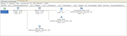
Figure 1

Starting from the right, as usual, we see a Clustered Index Scan operator, which gets the list of States based on the parameter, @CountryRegionCode, visible in the ToolTip or the Properties window. This data is then placed into an ordered state by the Sort operator. Data from the SalesTaxRate table is gathered using an Index Seek operator as part of the Nested Loop join with the sorted data from the States table.

Next, we have a Key Lookup operator. This operator takes a list of keys, like those supplied from Index Seek on the AK_CountryRegion_Name index from the SalesTaxRate table, and gets the data from where it is stored, on the clustered index. This output is joined to the output from the previous Nested Loop within another Nested Loop join for the final output to the user.

While this plan isn’t complex, the interesting point is that we don’t have a stored procedure in sight. Instead, the T-SQL within the stored procedure is treated in the same way as if we had written and run the SELECT statement through the Query window.

Derived Tables

One of the ways that data is accessed through T-SQL is via a derived table. If you are not familiar with derived tables, think of a derived table as a virtual table that’s created on the fly from within a SELECT statement.

You create derived tables by writing a second SELECT statement within a set of parentheses in the FROM clause of an outer SELECT query. Once you apply an alias, this SELECT statement is treated as a table. In my own code, one place where I’ve come to use derived tables frequently is when dealing with data that changes over time, for which I have to maintain history.

A Subselect without a Derived Table

Using AdventureWorks as an example, the Production.ProductionListPriceHistory table maintains a running list of changes to product price. To start with, we want to see what the execution plan looks like not using a derived table so, instead of a derived table, we’ll use a subselect within the ON clause of the join to limit the data to only the latest versions of the ListPrice.

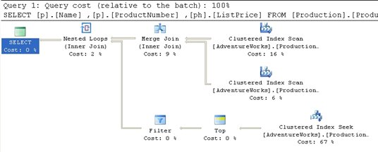
Figure 2

What appears to be a somewhat complicated query turns out to have a fairly straightforward execution plan. First, we get the two Clustered Index Scans against Production.Product and Production.­ProductListPriceHistory. These two data streams are combined using the Merge Join operator.

The Merge Join requires that both data inputs be ordered on the join key, in this case, ProductId. The data resulting from a clustered index is always ordered, so no additional operation is required here.

A Merge Join takes a row each from the two ordered inputs and compares them. Because the inputs are sorted, the operation will only scan each input one time (except in the case of a many-to-many join; more on that further down). The operation will scan through the right side of the operation until it reaches a row that is different from the row on the left side. At that point it will progress the left side forward a row and begin scanning the right side until it reaches a changed data point. This operation continues until all the rows are processed. With the data already sorted, as in this case, it makes for a very fast operation.

Although we don’t have this situation in our example, Merge Joins that are many-to-many create a worktable to complete the operation. The creation of a worktable adds a great deal of cost to the operation although it will generally still be less costly than the use of a Hash Join, which is the other choice the query optimizer can make. We can see that no worktable was necessary here because the ToolTips property labeled Many-To-Many (see figure below) that is set to “False”.

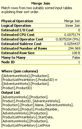
Figure 3

Next, we move down to the Clustered Index Seek operation in the lower right. Interestingly enough, this process accounts for 67% of the cost of the query because the seek operation returned all 395 rows from the query, only limited to the TOP (1) after the rows were returned. A scan in this case may have worked better because all the rows were returned. The only way to know for sure would be to add a hint to the query to force a table scan and see if performance is better or worse.

The Top operator simply limits the number of returned rows to the value supplied within the query, in this case “1.”

The Filter operator is then applied to limit the returned values to only those where the dates match the main table. In other words, a join occurred between the [Production].[Product] table and the [Production].[ProductListPriceHistory] table, where the column [StartDate] is equal in each. See the ToolTip in Figure 4:

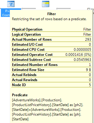
Figure 4

The two data feeds are then joined through a Nested Loops operator, to produce the final result.

A Derived Table using APPLY

Now that we have seen what kind of execution plan is created when using a subselect, we can rewrite the query to use a derived table instead. There are several different ways to do this, but we’ll look at how the SQL Server 2005 APPLY operator can be used to rewrite the above subselect into a derived query, and then see how this affects the execution plan.

SQL Server 2005 introduces a new type of derived table, created using one of the two forms of the APPLY operator, CROSS APPLY or OUTER APPLY. The APPLY operator allows you to use a table valued function, or a derived table, to compare values between the function and each row of the table to which the function is being “applied”.

If you are not familiar with the APPLY operator, check out: Using APPLY

Below is an example of the rewritten query. Remember, both queries return identical data, they are just written differently.

The introduction of this new functionality changes the execution plan substantially, as shown in Figure 5:

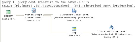
Figure 5

The TOP statement is now be applied row-by-row within the control of the APPLY functionality, so the second index scan against the ProductListPriceHistory table, and the merge join that joined the tables together, are no longer needed. Furthermore, only the Index Seek and Top operations are required to provide data back for the Nested Loops operation.

So which method of writing this query is more efficient? One way to find out is to run each query with the SET STATISTICS IO option set to ON. With this option set, IO statistics are displayed as part of the Messages returned by the query.

When we run the first query, which uses the subselect, the results are:

If we run the query using a derived table, the results are:

Although both queries returned identical result sets, the query with the subselect query uses fewer logical reads (795) verses the query written using the derived table (1008 logical reads).

This gets more interesting if we add the following WHERE clause to each of the previous queries:

When we re-run the original query with the added WHERE clause, we get the plan shown in Figure 6:

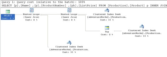
Figure 6

The Filter operator is gone but, more interestingly, the costs have changed. Instead of index scans and the inefficient (in this case) index seeks mixed together, we have three, clean Clustered Index Seeks with an equal cost distribution.

If we add the WHERE clause to the derived table query, we see the plan shown in Figure 7:

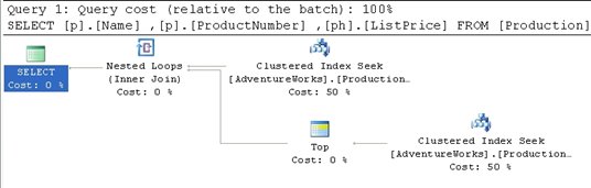
Figure 7

The plan is almost identical to the one seen in Figure 5, with the only change being that the Clustered Index Scan has changed to a Clustered Index Seek, because the inclusion of the WHERE clause allows the optimizer to take advantage of the clustered index to identify the rows needed, rather than having to scan through them all in order to find the correct rows to return.

Now, let’s compare the IO statistics for each of the queries, which return the same physical row.

When we run the query with the subselect, we get:

When we run the query with the derived query, we get:

Now, with the addition of a WHERE clause, the derived query is more efficient, with only 2 logical reads, versus the subselect query with 4 logical reads.

The lesson to learn here is that in one set of circumstances a particular T-SQL method may be exactly what you need, and yet in another circumstance that same syntax impacts performance. The Merge join made for a very efficient query when we were dealing with inherent scans of the data, but was not used, nor applicable, when the introduction of the WHERE clause reduced the data set. With the WHERE clause in place the subselect became, relatively, more costly to maintain when compared to the speed provided by the APPLY functionality. Understanding the execution plan makes a real difference in deciding which of these to apply.

Common Table Expressions

SQL Server 2005 introduced a T-SQL command, whose behavior appears similar to derived tables, called a common table expression (CTE). A CTE is a “temporary result set” that exists only within the scope of a single SQL statement. It allows access to functionality within that single SQL statement that was previously only available through use of functions, temp tables, cursors, and so on. Unlike derived tables, a CTE can be self referential and can be referenced repeatedly within a single query. For more details on the CTE check out this article in Simple-Talk: http://www.simple-talk.com/sql/sql-server-2005/sql-server-2005-common-table-expressions/.

One of the classic use cases for a CTE is to create a recursive query. AdventureWorks takes advantage of this functionality in a classic recursive exercise, listing employees and their managers. The procedure in question, uspGetEmployeeManagers, is as follows:

Let’s execute this procedure, capturing the actual XML plan:

We get a fairly complex execution plan so let’s break it down into sections in order to evaluate it. We will examine the XML plan alongside the graphical plan.

The top-right hand section of the graphical plan is displayed in Figure 8:

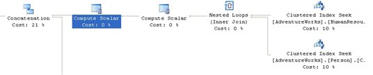
Figure 8

A Nested Loops join takes the data from Clustered Index Seeks against HumanResources.Employee and Person.Contact. The Scalar operator puts in the constant “0” from the original query for the derived column, RecursionLevel, since this is the core query for the common table expression.  The second scalar, which is only carried to a later operator, is an identifier used as part of the Concatenation operation.

This data is fed into a Concatenation operator. This operator scans multiple inputs and produces one output. It is most-commonly used to implement the UNION ALL operation from T-SQL.

The bottom right hand section of the plan is displayed in Figure 9:

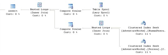
Figure 9

This is where things get interesting. The recursion methods are implemented via the Table Spool operator. This operator provides the mechanism for looping through the records multiple times. As noted in my previous article, this operator takes each of the rows and stores them in a hidden temporary object stored in the tempdb database. Later in the execution plan, if the operator is rewound (say due to the use of a Nested Loops operator in the execution plan) and no rebinding is required, the spooled data can be reused instead of having to rescan the data again. As the operator loops through the records they are joined to the data from the tables as defined in the second part of the UNION ALL definition within the CTE.

If you look up NodeId 19 in the XML plan, you can see the RunTimeInformation element.

This shows us that one rebind of the data was needed. The rebind, a change in an internal parameter, would be the second manager. From the results, we know that three rows were returned; the initial row and two others supplied by the recursion through the management chain of the data within Adventureworks.

The final section of the graphical plan is shown in Figure 10:

Figure 10

After the Concatenation operator we get an Index Spool operator. This operation aggregates the rows into a work table, within tempdb. The data gets sorted and then we just have the rest of the query, joining index seeks to the data put together by the recursive operation.

Views

A view is essentially just a “stored query” – a way of representing data as if it were a table, without actually creating a new table. The various uses of views are well documented (preventing certain columns being selected, reducing complexity for end users, and so on). Here, we will just focus on what happens within the execution plan when we’re working with a view.

Standard Views

The view, Sales.vIndividualCustomer, provides a summary of customer data, displaying information such as their name, email address, physical address and demographic information. A very simple query to get a specific customer would look something like this:

The resulting graphical execution plan is shown in Figure 11:

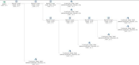
Figure 11

What happened to the view, vIndividualCustomer, which we referenced in this query? Remember that while SQL Server treats views similarly to tables, a view is just a named construct that sits on top of the component tables that make them up. The optimizer, during binding, resolves all those component parts in order to arrive at an execution plan to access the data. In effect, the query optimizer ignores the view object, and instead deals directly with the eight tables and the seven joins that are defined within this view.

This is important to keep in mind since views are frequently used to mask the complexity of a query. In short, while the view makes coding easier, it doesn’t in any way change the necessities of the query optimizer to perform the actions defined within the view.

Indexed Views

An Indexed View, also called a materialized view, is essentially a “view plus a clustered index”. A clustered index stores the column data as well as the index data, so creating a clustered index on a view results, essentially, in a new table in the database. Indexed views can often speed the performance of many queries, as the data is directly stored in the indexed view, negating the need to join and lookup the data from multiple tables each time the query is run.

Creating an indexed view is, to say the least, a costly operation. Fortunately, this is a one-time operation that can be scheduled to occur when your server is less busy.

Maintaining an index view is a different story. If the tables in the indexed view are relatively static, there is not much overhead associated with maintaining indexed views. On the other hand, if an indexed view is based on tables that are modified often, there can be a lot of overhead associated with maintaining the indexed view. For example, if one of the underlying tables is subject to a hundred INSERT statements a minute, then each INSERT will have to be updated in the indexed view. As a DBA, you have to decide if the overhead associated with maintaining an indexed view is worth the gains provided by creating the indexed view in the first place.

Queries that contain aggregates are a good candidate for indexed views because the creation of the aggregates can occur once, when the index is created, and the aggregated results can be returned with a simple SELECT query, rather than having the added overhead of running the aggregates through a GROUP BY each time the query runs.

For example, one of the indexed views supplied with AdventureWorks is vStateProvinceCountryRegion. This combines the StateProvince table and the CountryRegion table into a single entity for querying:

The execution plan is shown in Figure 12:

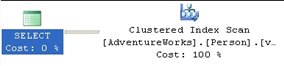
Figure 12

From our previous experience with execution plans containing views, you might have expected to see two tables and the join in the execution plan. Instead, we see a single Clustered Index Scan operation: rather than execute each step of the view, the optimizer went straight to the clustered index that makes this an indexed view.

Since these indexes are available to the optimizer, they can also be used by queries that don’t refer to the indexed view at all. For example, the following query will result in the exact same execution plan as shown in Figure 12:

This is because the optimizer recognizes the index as the best way to access the data.

However, this behavior is neither automatic nor guaranteed as execution plans become more complicated. For example, take the following query:

If you expected to see a join between the indexed view and the Person.Address table, you will be disappointed:

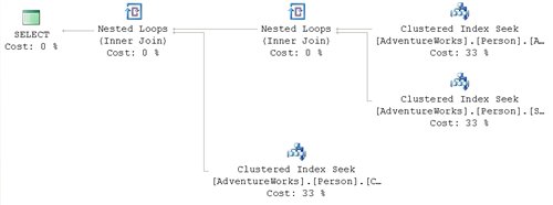
Figure 13

Instead of using the clustered index that defines the materialized view, as we saw in figure 12, the optimizer performs the same type of index expansion as it did when presented with a regular view. The query that defines the view is fully resolved, substituting the tables that make it up instead of using the clustered index provided with the view. There is a way around this, which will be explained when we encounter the NOEXPAND hint, in the Table Hints section of Chapter 5 in my book

Indexes

A big part of any tuning effort revolves around choosing the right indexes to include in a database. In most peoples’ minds, the importance of using indexes is already well established. A frequently asked question however, is “how come some of my indexes are used and others are not?”

The availability of an index directly affects the choices made by the query optimizer. The right index leads the optimizer to the selection of the right plan. However, a lack of indexes or, even worse, a poor choice of indexes, can directly lead to poor execution plans and inadequate query performance.

Included Indexes: Avoiding Bookmark Lookups

One of the more pernicious problems when attempting to tune a query is the Bookmark Lookup. Type “avoid bookmark lookup” into Google and you’ll get quite a few hits. As we discovered in my previous article, SQL Server 2005 no longer refers directly to bookmark lookup operators, although it does use the same term for the operation within its documentation.

To recap, a Bookmark Lookup occurs when a non-clustered index is used to identify the row, or rows, of interest, but the index is not covering (does not contain all the columns requested by the query). In this situation, the Optimizer is forced to send the Query Engine to a clustered index, if one exists (a Key Lookup), otherwise, to the heap, or table itself (a RID Lookup), in order to retrieve the data.

A Bookmark Lookup is not necessarily a bad thing, but the operation required to first read from the index followed by an extra read to retrieve the data from the clustered index, or heap, can lead to performance problems.

We can demonstrate this with a very simple query:

This query returns an execution plan, shown in Figure 14, which fully demonstrates the cost of lookups.

Figure 14

The Index Seek operator pulls back the four rows we need, quickly and efficiently. Unfortunately, the only data available on that index is the ProductId.

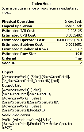
Figure 15

As you can see from figure 15, the index seek also outputs columns that define the clustered index, in this case SalesOrderId and SalesOrderDetailId. These are used to keep the index synchronized with the clustered index and the data itself.

We then get the Key LookUp, whereby the optimizer retrieves the other columns required by the query, OrderQty and UnitPrice, from the clustered index.

In SQL Server 2000, the only way around this would be to modify the existing index used by this plan, IX_SalesOrderDetail_ProductId, to use all three columns. However, in SQL Server 2005, we have the additional option of using the INCLUDE attribute within the non-clustered index.

The INCLUDE attribute was added to indexes in SQL Server 2005 specifically to solve problems of this type. It allows you to add a column to the index, for storage only, not making it a part of the index itself, therefore not affecting the sorting or lookup values of the index. Adding the columns needed by the query can turn the index into a covering index, eliminating the need for the lookup operation. This does come at the cost of added disk space and additional overhead for the server to maintain the index, so due consideration must be paid prior to implementing this as a solution.

In the following code, we create a new index using the INCLUDE attribute. In order to get an execution plan focused on what we’re testing, we set STATISTICS XML to on, and turn it off when we are done. The code that appears after we turn STATISTICS XML back off recreates the original index so that everything is in place for any further tests down the road.

Run this code in Management Studio with the “Include Actual Execution Plan” option turned on, and you will see the execution plan shown in Figure 16:

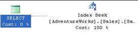
Figure 16

The execution plan is able to use a single operator to find and return all the data we need because the index is now covering, meaning it includes all the necessary columns.

Index Selectivity

Let’s now move on to the question of which index is going to get used, and why the optimizer sometimes avoids using available indexes.

First, let’s briefly review the definition of the two kinds of available indexes: the clustered and non-clustered index. A clustered index stores the data along with the lookup values of the index and it sorts the data, physically. A non-clustered index sorts the column, or columns, included in the index, but it doesn’t sort the data.

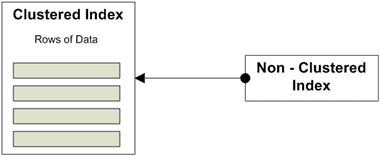
Figure 17

As described in my book, the utility of a given index is determined by the statistics generated automatically by the system for that index. The key indicator of the usefulness of the index is its selectivity.

An index’s selectivity describes the distribution of the distinct values within a given data set. To put it more simply, you count the number of rows and then you count the number of unique values for a given column across all the rows. After that, divide the unique values by the number of rows. This results in a ratio that is expressed as the selectivity of the index. The better the selectivity, the more useful the index and the more likely it will be used by the optimizer.

For example, on the Sales.SalesOrderDetail table there is an index, IX_SalesOrderDetail_ProductID, on the ProductID column. To see the statistics for that index use the DBCC command, SHOW_STATISTICS:

This returns three result sets with various amounts of data. Usually, the second result set is the most interesting one:

The Density is inverse to the selectivity, meaning that the lower the density, the higher the selectivity. So an index like the one above, with a density of .003759399, will very likely be used by the optimizer. The other rows refer to the clustered index. Any index in the system that is not clustered will also have a pointer back to the clustered index since that’s where the data is stored. If no clustered index is present then a pointer to the data itself, often referred to as a heap, is generated. That’s why the columns of the clustered index are included as part of the selectivity of the index in question.

Selectivity can affect the use of an index negatively as well as positively. Let’s assume that you’ve taken the time to create an index on a frequently-searched field, and yet you’re not seeing a performance benefit. Let’s create such a situation ourselves. The business represented in AdventureWorks has decided that they’re going to be giving away prizes based on the quantity of items purchased. This means a query very similar to the one from the previous Avoiding BookMark Lookups section:

The execution plan for this query is shown in Figure 18:

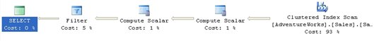
Figure 18

We see a Clustered Index Scan against the entire table and then a simple Filter operation to derive the final results sets, where OrderQty = 10.

Let’s now create an index that our query can use:

Unfortunately, if you capture the plan again, you’ll see that it’s identical to the one shown in Figure 18; in other words, our new index is completely ignored. Since we know that selectivity determines when, or if, and index is used, let’s examine the new index using DBCC SHOW_STATISTICS:

We can see that the density of the OrderQty is 10 times less than for the ProductId column, meaning that our OrderQty index is ten times less selective. To see this in more quantifiable terms, there are 121317 rows in the SalesOrderDetail table on my system. There are only 41 distinct values for the OrderQty column. This column just isn’t, by itself, an adequate index to make a difference in the query plan.

If we really had to make this query run well, the answer would be to make the index selective enough to be useful by the optimizer. You could also try forcing the optimizer to use the index we built by using a query hint, but in this case, it wouldn’t help the performance of the query (hints are covered in detail in Chapter 5 of my book). Remember that adding an index, however selective, comes at a price during inserts, deletes and updates as the data within the index is reordered, added or removed based on the actions of the query being run.

If you’re following along in AdventureWorks, you’ll want to be sure to drop the index we created:

Statistics and Indexes

The main cause of a difference between the plans lies in differences between the statistics and the actual data. Not only can this cause differences between the plans, but you can get bad execution plans because the statistical data is not up to date.

The following example is somewhat contrived, but it does demonstrate how, as the data changes, the exact same query will result in two different execution plans. In the example, the new table is created, along with an index:

I then capture the estimated plan (in MXL format). After that I run a query that updates the data, changing the statistics and then run another query, getting the actual execution plan

I took the XML output and saved them to files (See Saving XML Plans as Graphical Plans, in Chapter 1 of my book), and then reopened the files in order to get an easy-to-read graphical plan. Breaking bits and pieces of SQL code apart and only showing plans for the pieces that you want is a big advantage to using XML plans. First the estimated plan:

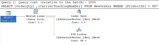
Figure 19

Then the Actual execution plan:

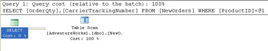
Figure 20

Go to the top and right of Figure 19 to find the Index Seek operator. Clearly, prior to the updates, the data and statistics within the index were selective enough that the SELECT could use a seek operation. Then, because the data being requested is not included in the index itself, a RID Lookup operation is performed. This is a lookup against a heap table using the row identifier to bring back the data from the correct row.

However, after the data is updated, the query is much less selective and returns much more data, so that the actual plan does not use the index, but instead retrieves the data by scanning the whole table, as we can see from the Table Scan operator in Figure 20. The estimated cost is .243321 while the actual cost is 1.2434. Note that if you recapture the estimated plan, you’ll see that the statistics have automatically updated, and the estimated plan will also show a table scan.

Summary

This article introduced various concepts that go a bit beyond the basics in displaying and understanding execution plans. Stored procedures, views, derived tables, and common table expressions were all introduced along with their attendant execution plans.

The most important point to take away from all of the various plans derived is that you have to walk through them all in the same way, working right to left, top to bottom, in order to understand the behavior implied by the plan. The importance of indexes and their direct impact on the execution of the optimizer and the query engine was introduced. The most important point to take away from here is that simply adding an index doesn’t necessarily mean you’ve solved a performance problem. You need to ensure the selectivity of your data. You also need to make appropriate choices regarding the addition or inclusion of columns in your indexes, both clustered and non-clustered.