
Hi there. Recently, I’ve been suffering from an existential crisis called “Optimizer rocks! Not!”. Let me try to explain it.
There are several stages of working with, and studying, the SQL Server query optimizer (or the equivalent from any other database technology). Each of these stages has its associated emotional conflicts based on the learning experience. Here are the stages and their emotional reactions, from my own experience:
- Umm, if I press CTRL+L I can see some nice colored icons. I wonder what they do?
- I’ve to learn how to read an execution plan and stop referring to them as colored icons.
- What on Earth does this operator do?
- Why does it do that? Please can someone help me to understand?
- Conor Cunningham is awesome: What a nice guy!
- Aaaaah, I’m starting to understand how it works.
- What distant planet did Paul White originally come from?
- Wow! What a smart piece of software the optimizer is!
- I envy Paul White‘s brain so much that my teeth are grinding together.
- Oops, the query optimizer is not estimating properly!
- Hmm. Maybe I can do something to improve this query plan 1!
- Ah! I think I can do something to improve this query plan 2!
- Ahhh, I feel sure I can do something to improve this query plan 3!
- Statistics rocks! Not!
- Joins rocks! Not!
- The Optmizer rocks! Not!
- …
Yep, I’m on the “optimizer rocks! Not!” stage. I’m not sure what the next stages are…
I don’t know why, it could just be my luck, but recently 60% of the queries that I’m tuning have turned out to have a bad execution plan. OK, I know that in most cases this isn’t a fault of the query optimizer, but that of the over-evolved ape at the keyboard. It is the human being that is generally responsible for the query optimizer’s mistakes by, for example, forgetting to update the statistics or writing a non-sarg. But apart from those cases, I’m still occasionally finding that the query optimizer is responsible for creating a bad query plan.
Look, I’m not saying this is a problem or a bug in the SQL Server optimizer in particular, because all database optimizers have their limits. There are often so many possible plans for a single query that it is impossible to analyze all of the possible alternatives to pick the best one, the one with the lowest cost. I understand all that, and I think that the SQL Server query optimizer is awesome!
The SQL Server query optimizer is based on a framework called Cascades [2] and it performs a significant number of explorations when it is trying to achieve a plan that is “good enough”. This plan should be created using as few resources as possible, and in the fastest possible time. On SQL Server, these explorations have many stages that are performed sequentially. One of the first stages performs the “heuristic join reorder” where the optimizer tries to identify the order in which the joins of a query will be executed. The main challenge of optimizing a query is to do this in the least time with the greatest efficiency possible. In a perfect world the optimizer should never take more time to optimize a query than it will take to execute it. It may seem trivial but, trust me, it isn’t. The number of possible permutations to join a 12-table query would be nearly 479 million, and if we consider bushy plans as an alternative we’ll end up with 28 trillion permutations. In other words, it is impossible to assess all of the plans to see which one is the best (see reference 5 for more information).
Having said all of that, I ought to make it clear that I don’t want to show the inefficiency of SQL Server query optimizer with this article. I want to show you that the search space of optimizing query is always harder and more complicated than it looks, and sometimes we can do things to help it to create better plans.
SQL Server Bushy Plans
For many years, I’ve being trying to create a real and practical example as an excuse to talk about bushy plans (look the references for more information) on SQL Server. In brief, a bushy plan is one of the options that SQL Server can consider when working out the best way to execute the joins of your query. To perform a join operation, the optimizer considers many ordering alternatives to access the tables of your query. This order can follow a left-deep tree where the result of the join is used as an outer input for the next join; Alternatively, it can use a right-deep tree where the result of the join is used as an inner input for the next join (look at the image below to see a graphical sample).
Actually, when optimizing a query the SQL Server optimizer considers only the options I’ve described above, but there is another option that isn’t used by default, which is the bushy tree.
Bushy trees can be interesting in cases where a join performs a good filtering of the resultset: In other words, you read lot of rows but, after performing the join, just a few rows are returned. A bushy plan, a plan with a bushy tree, can be a plan that performs a join based on the result of two other joins. Consider the following query:
|
1 2 3 4 5 |
SELECT * FROM A JOIN B ON A.ID = B.ID JOIN C ON A.ID = C.ID JOIN D ON A.ID = D.ID |
We could have the following plans:
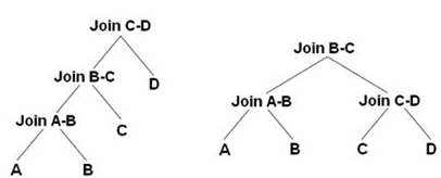
Picture from Benjamin Nevarez’ blog post
The first tree is a plan using a left-deep tree that executes the join in the following order:
- JOIN( JOIN( JOIN(A, B), C), D)
The second tree is a plan using a bushy-tree that executes the join in the following order:
- JOIN(JOIN(A, B), JOIN(C, D))
The SQL Server optimizer doesn’t consider the possibility of using bushy trees because it could be very expensive to do it so. In order to force a bushy plan, we’ve got two options: We can either use a CTE as I’ll show you, or use a weird syntax to join the tables (see References at the bottom of this article and Itzik’s blog post in particular for more details). Both these options require you to use the FORCE ORDER query hint.
Now that you understand a little about bushy plans, let me show you a practical example of optimization that we can do. Our test will be based on the Northwind database. To illustrate it, let’s start by creating some large tables:
|
1 2 3 4 5 6 7 8 9 10 11 12 13 14 15 16 17 18 19 20 21 22 23 24 25 26 27 28 29 30 31 32 33 34 35 36 37 38 39 40 41 42 43 44 45 46 47 48 49 50 51 52 53 54 55 |
USE NorthWind GO IF OBJECT_ID('OrdersBig') IS NOT NULL DROP TABLE OrdersBig GO SELECT TOP 5000000 IDENTITY(Int, 1,1) AS OrderID, ABS(CheckSUM(NEWID()) / 10000000) AS CustomerID, CONVERT(Date, GETDATE() - (CheckSUM(NEWID()) / 1000000)) AS OrderDate, ISNULL(ABS(CONVERT(Numeric(18,2), (CheckSUM(NEWID()) / 1000000.5))),0) AS Value INTO OrdersBig FROM Orders A CROSS JOIN Orders B CROSS JOIN Orders C CROSS JOIN Orders D GO ALTER TABLE OrdersBig ADD CONSTRAINT xpk_OrdersBig PRIMARY KEY(OrderID) GO IF OBJECT_ID('CustomersBig') IS NOT NULL DROP TABLE CustomersBig GO SELECT TOP 5000000 IDENTITY(Int, 1,1) AS CustomerID, SubString(CONVERT(VarChar(250),NEWID()),1,20) AS CompanyName, SubString(CONVERT(VarChar(250),NEWID()),1,20) AS ContactName, CONVERT(VarChar(250), NEWID()) AS Col1, CONVERT(VarChar(250), NEWID()) AS Col2 INTO CustomersBig FROM Customers A CROSS JOIN Customers B CROSS JOIN Customers C CROSS JOIN Customers D GO ALTER TABLE CustomersBig ADD CONSTRAINT xpk_CustomersBig PRIMARY KEY(CustomerID) GO IF OBJECT_ID('ProductsBig') IS NOT NULL DROP TABLE ProductsBig GO SELECT TOP 5000000 IDENTITY(Int, 1,1) AS ProductID, SubString(CONVERT(VarChar(250),NEWID()),1,20) AS ProductName, CONVERT(VarChar(250), NEWID()) AS Col1 INTO ProductsBig FROM Products A CROSS JOIN Products B CROSS JOIN Products C CROSS JOIN Products D GO ALTER TABLE ProductsBig ADD CONSTRAINT xpk_ProductsBig PRIMARY KEY(ProductID) GO IF OBJECT_ID('Order_DetailsBig') IS NOT NULL DROP TABLE Order_DetailsBig GO SELECT OrdersBig.OrderID, ISNULL(CONVERT(Integer, CONVERT(Integer, ABS(CheckSUM(NEWID())) / 1000000)),0) AS ProductID, GetDate() - ABS(CheckSUM(NEWID())) / 1000000 AS Shipped_Date, CONVERT(Integer, ABS(CheckSUM(NEWID())) / 1000000) AS Quantity INTO Order_DetailsBig FROM OrdersBig GO ALTER TABLE Order_DetailsBig ADD CONSTRAINT [xpk_Order_DetailsBig] PRIMARY KEY([OrderID], [ProductID]) GO |
We’ll then create these indexes:
|
1 2 3 4 5 |
CREATE INDEX ixContactName ON CustomersBig(ContactName) -- indexing WHERE CREATE INDEX ixProductName ON ProductsBig(ProductName) -- indexing WHERE CREATE INDEX ixCustomerID ON OrdersBig(CustomerID) INCLUDE(Value) -- indexing FK CREATE INDEX ixProductID ON Order_DetailsBig(ProductID) INCLUDE(Quantity) -- indexing FK GO |
Now let’s insert a new order for a new customer:
|
1 2 3 4 5 6 7 8 9 10 11 |
-- create new customer INSERT INTO CustomersBig (CompanyName, ContactName, Col1, Col2) VALUES ('Emp Fabiano', 'Fabiano Amorim', NEWID(), NEWID()) -- Insert order to new customer INSERT INTO OrdersBig (CustomerID, OrderDate, Value) VALUES(SCOPE_IDENTITY(), GetDate(), 999) SET IDENTITY_INSERT Order_DetailsBig ON INSERT INTO Order_DetailsBig(OrderID, ProductID, Shipped_Date, Quantity) VALUES (SCOPE_IDENTITY(), 1, GetDate() + 30, 999) SET IDENTITY_INSERT Order_DetailsBig OFF GO |
And finally, the following query returns some information about the sales to the Customer ‘Fabiano Amorim’ for a specific Product:
|
1 2 3 4 5 6 7 8 9 10 11 12 13 14 15 16 17 18 |
-- "cold cache" CHECKPOINT; DBCC FREEPROCCACHE; DBCC DROPCLEANBUFFERS; GO SELECT OrdersBig.OrderID, OrdersBig.Value, Order_DetailsBig.Quantity, CustomersBig.ContactName, ProductsBig.ProductName FROM OrdersBig INNER JOIN CustomersBig ON OrdersBig.CustomerID = CustomersBig.CustomerID INNER JOIN Order_DetailsBig ON OrdersBig.OrderID = Order_DetailsBig.OrderID INNER JOIN ProductsBig ON Order_DetailsBig.ProductID = ProductsBig.ProductID WHERE CustomersBig.ContactName = 'Fabiano Amorim' AND ProductsBig.ProductName = 'E1033B5D-EAC8-41FF-B' GO |
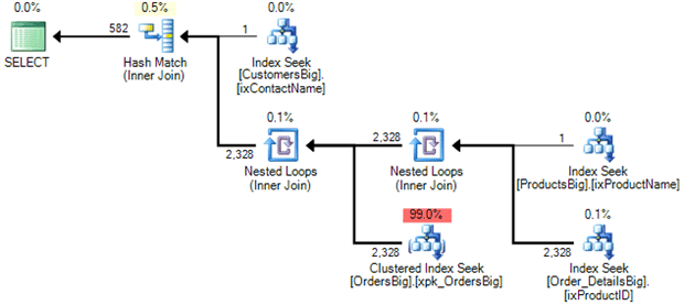
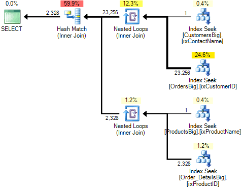
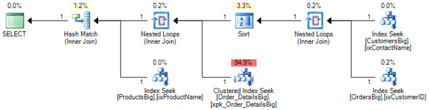
We’ve got the following plan:
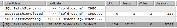
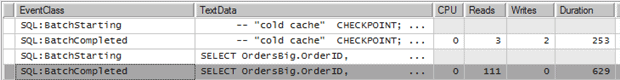
And the performance we get from the query is:
Statistics IO:
|
1 2 3 4 5 |
Table 'Worktable'. Scan count 0, logical reads 0, physical reads 0, read-ahead reads 0 Table 'OrdersBig'. Scan count 0, logical reads 11835, physical reads 1, read-ahead reads 11792 Table 'Order_DetailsBig'. Scan count 1, logical reads 10, physical reads 1, read-ahead reads 7 Table 'ProductsBig'. Scan count 1, logical reads 3, physical reads 3, read-ahead reads 0 Table 'CustomersBig'. Scan count 1, logical reads 3, physical reads 3, read-ahead reads 0 |
As we can see from the statistics io result, there is a big problem with this plan to do with the order in which the joins will be executed. If we follow the join ordering, the seek on OrdersBig will be executed hundreds of times. As we can see in the plan, it is estimating that 2328 seeks will be executed on OrdersBig. That is the number of rows being returned from the join between ProductsBig and OrderDetails_Big.
Since we know that there is only one order for customer “Fabiano Amorim”, why not to join CustomersBig with OrdersBig ? Why to choose to Join ProductsBig and OrderDetails_Big, before then joining the result with OrdersBig? If the query optimizer had chosen a plan that joins CustomersBig + OrdersBig, then only one seek on OrdersBig would be needed.
This bad estimate happened because, at the time that the plan was compiled, the query optimizer doesn’t know the value of CustomerID for the customer “Fabiano Amorim” and so it can’t use the histogram statistic for OrdersBig.CustomerID column to estimate that only one row matches with CustomerID of “Fabiano Amorim”.
If this example is too confusing, then let me try to use another example. Let’s suppose that we have the following query:
|
1 2 3 4 5 |
SELECT OrdersBig.OrderID, CustomersBig.ContactName FROM OrdersBig INNER JOIN CustomersBig ON OrdersBig.CustomerID = CustomersBig.CustomerID WHERE CustomersBig.ContactName = 'Fabiano Amorim' |
Estimated query plan:
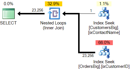
Notice that the estimated number of rows that will be returned for the customer “Fabiano Amorim” on CustomersBig is just one row, but after the seek of the table OrdersBig, it is estimating that 23256 rows will be returned – crazy, huh? Yep, this is a ‘known problem’ for the query optimizer. At compilation-plan time, the optimizer doesn’t yet know the value that will be returned for CustomersBig.CustomerID and so it can’t estimate how many numbers it will return from OrdersBig, so what does it do? It uses the density of the column OrdersBig.CustomerID.
Multi-Column Cross-Table Statistics would help a lot on this case, but we haven’t got it in SQL Server yet. Another way to help with estimation statistics would be to create a filtered statistic on CustomersBig, something like “CREATE STATISTICS stats1 ON CustomersBig(CustomerID) WHERE ContactName = ‘Fabiano Amorim'” but that will have to be the subject for another article.
Just to make it clear how the optimizer used the density to get to the number 23256, let’s dig into it a little bit. If we run:
|
1 |
sp_helpstats OrdersBig |
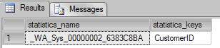
We’ve an auto-created a statistic based in the column CustomerID from OrdersBig table. This statistic was created by the optimizer to help to estimate how many rows will be returned from OrdersBig table. Let’s get more information about this statistic:
|
1 |
DBCC SHOW_STATISTICS (OrdersBig, _WA_Sys_00000002_6383C8BA) |
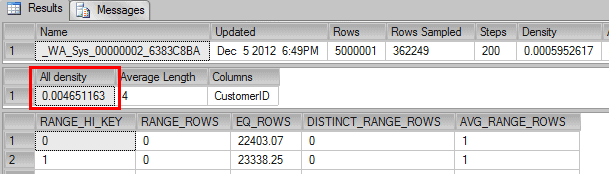
To estimate the number of rows returned by the seek on OrdersBig table, SQL Server used the following formula: density * number of rows in the table. That is, 0.004651163 * 5000000 = 23256 (rounding up) which is exactly the value used in the estimated query plan.
The same density estimation was used to estimate how many rows from the join between ProductsBig and OrderDetails_Big will be returned. In that case, the number that was estimated was very good: It is estimating that the number of rows returned from the seek on the Order_DetailsBig is 2328 rows and the actual number of rows is 2356, which is pretty close to the estimated figure.
Going back to the plan that we’re analyzing, we’ve found that because SQL Server has estimated that 23256 rows will be returned from a join on CustomersBig and OrdersBig, it chooses not to do it, but instead it prefers to join ProductsBig and OrderDetails_Big, then join the result with OrdersBig and finally join these results with CustomersBig.
“Ok Fabiano, but what do bushy plans have to do with it?”
Calm down, we’ll get there right now. Knowing that only one row will be returned from CustomersBig + OrdersBig, we could force a plan that follows this order of execution. The order using a bushy plan would be this:
|
1 |
JOIN(JOIN(CustomersBig, OrdersBig), JOIN(ProductsBig, Order_DetailsBig)) |
Let’s write a query using a CTE and the FORCE ORDER hint:
|
1 2 3 4 5 6 7 8 9 10 11 12 13 14 15 16 17 18 19 20 21 22 23 24 25 26 27 28 29 30 31 32 33 34 35 36 |
-- "cold cache" CHECKPOINT; DBCC FREEPROCCACHE; DBCC DROPCLEANBUFFERS; GO ;WITH JoinEntre_CustomersBig_e_OrdersBig AS ( SELECT OrdersBig.OrderID, OrdersBig.Value, CustomersBig.ContactName FROM CustomersBig INNER JOIN OrdersBig ON OrdersBig.CustomerID = CustomersBig.CustomerID ), JoinEntre_ProductsBig_e_Order_DetailsBig AS ( SELECT Order_DetailsBig.OrderID, Order_DetailsBig.Quantity, ProductsBig.ProductName FROM ProductsBig INNER JOIN Order_DetailsBig ON Order_DetailsBig.ProductID = ProductsBig.ProductID ) SELECT JoinEntre_CustomersBig_e_OrdersBig.OrderID, JoinEntre_CustomersBig_e_OrdersBig.Value, JoinEntre_ProductsBig_e_Order_DetailsBig.Quantity, JoinEntre_CustomersBig_e_OrdersBig.ContactName, JoinEntre_ProductsBig_e_Order_DetailsBig.ProductName FROM JoinEntre_CustomersBig_e_OrdersBig INNER JOIN JoinEntre_ProductsBig_e_Order_DetailsBig ON JoinEntre_CustomersBig_e_OrdersBig.OrderID = JoinEntre_ProductsBig_e_Order_DetailsBig.OrderID WHERE JoinEntre_CustomersBig_e_OrdersBig.ContactName = 'Fabiano Amorim' AND JoinEntre_ProductsBig_e_Order_DetailsBig.ProductName = 'E1033B5D-EAC8-41FF-B' OPTION (FORCE ORDER, MAXDOP 1) GO |
We’ve got the following query plan:
As you can see from the CTE code, I wrote the query in the exact order that I want SQL Server to follow and I also used the FORCE ORDER query hint to tell SQL Server to follow my order of writing the tables to create the plan. The result is that we’ve got a bushy plan that joins the results between two other join results. By doing this, we’ve ended up with a query that performs much better than the original plan created by query optimizer. Let’s see the performance:
Results from profiler: 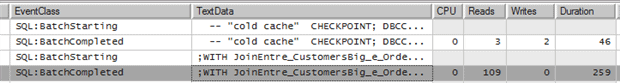
Statistics IO:
|
1 2 3 4 5 |
Table 'Worktable'. Scan count 0, logical reads 0, physical reads 0, read-ahead reads 0 Table 'Order_DetailsBig'. Scan count 1, logical reads 10, physical reads 1, read-ahead reads 7 Table 'ProductsBig'. Scan count 1, logical reads 3, physical reads 3, read-ahead reads 0 Table 'OrdersBig'. Scan count 1, logical reads 4, physical reads 1, read-ahead reads 8 Table 'CustomersBig'. Scan count 1, logical reads 3, physical reads 3, read-ahead reads 0 |
The performance difference is awesome. The first query runs in 6 seconds and the bushy plan query runs in 259 milliseconds and uses much less CPU and disk resources.
There is something important to remember: The fewer rows that we return from the joins, the better the performance of the bushy plan will be. For instance, if you run the query using a ProductName or a ContactName that does not exist, then the performance will be perfect.
Another option that I think worthy to mention is to use FORCE ORDER to create a plan that joins like JOIN(JOIN(JOIN(CustomersBig, OrdersBig), Order_DetailsBig), ProductsBig), for instance:
|
1 2 3 4 5 6 7 8 9 10 11 12 13 14 15 16 17 18 19 |
-- "cold cache" CHECKPOINT; DBCC FREEPROCCACHE; DBCC DROPCLEANBUFFERS; GO SELECT OrdersBig.OrderID, OrdersBig.Value, Order_DetailsBig.Quantity, CustomersBig.ContactName, ProductsBig.ProductName FROM CustomersBig INNER JOIN OrdersBig ON OrdersBig.CustomerID = CustomersBig.CustomerID INNER JOIN Order_DetailsBig WITH(FORCESEEK) ON OrdersBig.OrderID = Order_DetailsBig.OrderID INNER JOIN ProductsBig ON Order_DetailsBig.ProductID = ProductsBig.ProductID WHERE CustomersBig.ContactName = 'Fabiano Amorim' AND ProductsBig.ProductName = '277F4DFD-268D-4C4F-8' OPTION (FORCE ORDER, MAXDOP 1) GO |
We have the following execution plan:
This query works pretty well if you query just a few Orders, so let’s see the performance from profiler:
Statistics IO:
|
1 2 3 4 5 |
Table 'Worktable'. Scan count 0, logical reads 0, physical reads 0, read-ahead reads 0 Table 'Order_DetailsBig'. Scan count 1, logical reads 10, physical reads 1, read-ahead reads 7 Table 'ProductsBig'. Scan count 1, logical reads 3, physical reads 3, read-ahead reads 0 Table 'OrdersBig'. Scan count 1, logical reads 4, physical reads 1, read-ahead reads 8 Table 'CustomersBig'. Scan count 1, logical reads 3, physical reads 3, read-ahead reads 0 |
But if you query using a ProductName and ContactName with a lower selectivity this plan will not be as good – in fact it will be much worse compared to the bushy plan. As a sample you could try to query for a customer with many orders to see the performance difference.
Conclusions
Important note:
This article is merely illustrative and is based on a database that doesn’t have real data. The intention of this article is to present you with the technique of using bushy-plans and how it works, but it is up to you to find real production world scenarios that fit into this technique. As with many other hints, it isn’t a good practice to force a plan by using hints because what you are doing is limiting the query optimizer’s freedom to generate a plan based on the actual data that is present in the tables. Sometimes you can use it, but it requires a lot of investigation and periodic maintenance to the query to ensure that the things haven’t changed and if the forced plan is still valid.
The damage that a bad forced plan causes can be much worse than a bad plan created by the query optimizer, so please use it with extra caution.
Query tuning optimization has a lot of variables and often it can boil down to trial-and-error techniques. However, it is important to know and understand how query optimization works to minimize the work necessary for a query plan tuning.
I hope you had liked the article. I’ve worked with important concepts about the query optimizer. If you want to know more about them take a look at the references – I’m sure you’ll like them.
That’s all folks.
References:
- ACM Paper: Left-deep vs. bushy trees: an analysis of strategy spaces and its implications for query optimization
- G. Graefe. The Cascades framework for query optimization. Data Engineering Bulletin, 18(3), 1995.
- Microsoft Research: Polynomial Heuristics for Query Optimization
- Itzik Ben-Gan: T-SQL Deep Dives: Create Efficient Queries
- Benjamin Nevarez: Optimizing Join Orders
- Wikipedia: http://en.wikipedia.org/wiki/Query_optimizer
This document contains proprietary information and is protected by copyright law.
Copyright © 2026 Red Gate Software Limited. All rights reserved


Load comments