It is possible to impose your will on the optimizer and, to some degree, control its behavior. This is done through hints:

• Query Hints   tell the optimizer to apply this hint throughout the execution of the entire query.
• Join Hints   tell the optimizer to use a particular join at a particular point in the query
• Table Hints   control table scans and the use of a particular index for a table

In this article I’ll describe how to use each of the above types of hint, but I can’t stress the following hard enough: these things are dangerous. Appropriate use of the right hint on the right query can save your application. The exact same hint used on another query can create more problems than it solves, slowing your query down radically and leading to severe blocking and timeouts in your application.

If you find yourself putting hints on a majority of your queries and procedures, then you’re doing something wrong. Within the details of each of the hints described, I’ll lay out the problem that you’re hoping to solve by applying the hint. Some of the examples will improve performance or change the behavior in a positive manner, and some will negatively impact performance.

Query Hints 

There are quite a number of query hints and they perform a variety of different duties. Some may be used somewhat regularly and a few are for rare circumstances.

Query hints are specified in the OPTION clause. The basic syntax is as follows:

Query hints can’t be applied to INSERT statements except when used with a SELECT operation. You also can’t use query hints in subselect statements.

Before we proceed, let me take this opportunity to warn you once again: injudicious use of these hints can cause you more problems than they solve!

HASH|ORDER GROUP 

These two hints – HASH GROUP   or grouping to the aggregation, respectively.

In the example below we have a simple GROUP BY query that is called frequently by the application to display the various uses of Suffix to people’s names.

The business has instructed you to make this query run as fast as possible because you’re maintaining a high-end shop with lots of queries from the sales force against an ever-changing set of data. The first thing you do, of course, is to look at the execution plan, as shown in Figure 1:

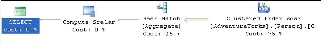
Figure   1

As you can see, by “default” the optimizer opts to use hashing   and then develop the counts based on the matched values. This plan has a cost of 0.590827, which you can see in the Tool Tip in Figure 2:

Figure   2

Since it’s not performing in the manner you would like, you decide that the best solution would be to try to use the data from the Clustered Scan in an ordered fashion rather than the unordered Hash Match   hint to the query:

The new plan is shown in Figure 3:

 

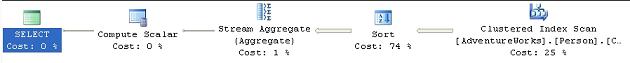
Figure 3

We’ve told the optimizer to use ordering rather than hashing   operator, which works with ordered data.

As per my repeated warning, this query had a cost of .590827 prior to applying the hint and a cost of 1.77745 after, a little more than three times the cost. The source of the increased cost is ordering the data as it comes out of the Clustered Index Scan  .

Depending on your situation, you may find an instance where, using our example above, the data is already ordered yet the optimizer chose to use the Hash Match  . In that case, the Query Engine would recognize that the data was ordered and accept the hint gracefully, increasing performance. While query hints allow you to control the behavior of the optimizer, it doesn’t mean your choices are necessarily better than those provided to you. To optimize this query, you may want to consider adding a different index or modifying the clustered index.

MERGE |HASH |CONCAT UNION 

These hints affect how UNION operations are carried out in your queries, instructing the optimizer to use either merging, hashing   or concatenation of the data sets. The most likely reason to apply this hint would be with performance issues where you may be able to affect the behavior of how the UNION is executed.

The example query below is not running fast enough to satisfy the demands of the application:

 

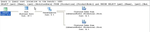
Figure 4

You can see that the Concatenation   operation that follows it is relatively expensive. The overall cost of the plan is 0.0377.

In a test to see if changing implementation of the UNION operation will affect overall performance, you apply the MERGE UNION   hint:

 

 

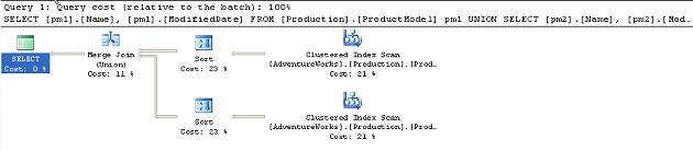
Figure 5

You have forced the UNION operation to use the Merge Join   operators. The estimated cost for the query has gone from 0.0377 to 0.0548. Clearly this didn’t work.

What if you tried the other hint, HASH UNION  :

This results in a new execution plan, shown in Figure 6:

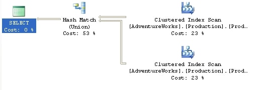
Figure 6

The execution plan is simplified, with the sort operations completely eliminated. However, the cost is still higher (0.0497) than for the original un-hinted query so clearly, for the amount of data involved in this query, the Hash Match   operator.

In this situation, the hints are working to modify the behavior of the query, but they are not helping you to increase performance of the query.

LOOP|MERGE|HASH JOIN 

This makes all the join operations in a particular query use the method supplied by the hint. However, note that if a join hint   (covered later in this article) is applied to a specific join, then the more granular join hint takes precedence over the general query hint.

You’ve found that your system is suffering from poor disk I/O, so you need to reduce the number of scans and reads that your queries generate. By collecting data from Profiler and Performance Monitor you’re able to identify the following query as needing some work. Here is the query and the original execution plan:

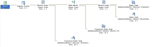
Figure 7

As you can see, the query uses a mix of Nested Loop  check box.

• Table ‘Contact’. Scan count 0, logical reads 1586, …

• Table ‘Worktable’. Scan count 0, logical reads 0, …

• Table ‘Address’. Scan count 1, logical reads 216, …

• Table ‘CustomerAddress’. Scan count 753, logical reads 1624, …

• Table ‘Store’. Scan count 1, logical reads 103, …

• Table ‘StoreContact’. Scan count 20, logical reads 42, …

• Table ‘ContactType’. Scan count 1, logical reads 2, …

From this data, you can see that the scans against the CustomerAddress table are causing a problem within this query. It occurs to you that allowing the query to perform all those Hash Join operations is slowing it down and you decide to change the behavior by adding the Loop Join hint to the end of the query:

 

Figure 8

Now the Hash Joins are Loop Joins  . This situation could be interesting. If you look at the operations that underpin the query execution plan you’ll see that the second query, with the hint, eliminates the creation of a work table. While the estimated cost of the second query is a bit higher than the original, the addition of the query hint does, in this case, results in a negligible improvement in performance, going from about 172ms to about 148ms on average. However, when you look at the scans and reads, they tell a different story:

• Table ‘ContactType’. Scan count 0, logical reads 1530, …

• Table ‘Contact’. Scan count 0, logical reads 1586, …

• Table ‘StoreContact’. Scan count 712, logical reads 1432, …

• Table ‘Address’. Scan count 0, logical reads 1477, …

• Table ‘CustomerAddress’. Scan count 701, logical reads 1512, …

• Table ‘Store’. Scan count 1, logical reads 103, …

Not only have we been unsuccessful in reducing the reads, despite the elimination of the work table, but we’ve actually increased the number of scans. What if we were to modify the query to use the MERGE JOIN hint instead? Change the final line of the query to read:

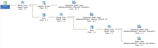
Figure 9

The execution of the plan was about as fast as the original, but did it solve our problem?

• Table ‘Worktable’. Scan count 11, logical reads 91, …

• Table ‘CustomerAddress’. Scan count 1, logical reads 6, …

• Table ‘StoreContact’. Scan count 1, logical reads 4, …

• Table ‘ContactType’. Scan count 1, logical reads 2, …

• Table ‘Store’. Scan count 1, logical reads 103, …

• Table ‘Address’. Scan count 1, logical reads 18, …

• Table ‘Contact’. Scan count 1, logical reads 33, …

We’ve re-introduced a worktable, but it does appear that the large number of scans has been eliminated. We may have a solution. However, before we conclude the experiment, we may as well as try out the HASH JOIN hint to see what it might do. Modify the final line of the query to read:

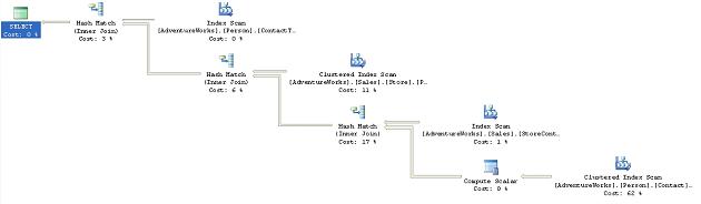
Figure 10

We’re back to a simplified execution plan using only Hash Join operations. The execution time was about the same as the original query and the I/O looked like this:

• Table ‘Worktable’. Scan count 0, logical reads 0, …

• Table ‘Contact’. Scan count 1, logical reads 569, …

• Table ‘Store’. Scan count 1, logical reads 103, …

• Table ‘Address’. Scan count 1, logical reads 216, …

• Table ‘CustomerAddress’. Scan count 1, logical reads 67, …

• Table ‘StoreContact’. Scan count 1, logical reads 4, …

• Table ‘ContactType’. Scan count 1, logical reads 2, …

For the example above, using the MERGE JOIN hint appears to be the best bet for reducing the I/O costs of the query, with only the added overhead of the creation of the worktable.

FAST n 

This time, we’re not concerned about performance of the database. This time, we’re concerned about perceived performance of the application. The users would like an immediate return of data to the screen, even if it’s not the complete result set, and even if they have to wait longer for the complete result set.

The FAST n   hint provides that feature by getting the optimizer to focus on getting the execution plan to return the first ‘n’ rows as fast as possible, where ‘n’ has to be a positive integer value. Consider the following query and execution plan:

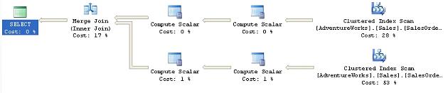
Figure 11

This query performs adequately, but there is a delay before the end users see any results, so we try to fix this by adding the Fast n hint to return the first 10 rows as quickly as possible:

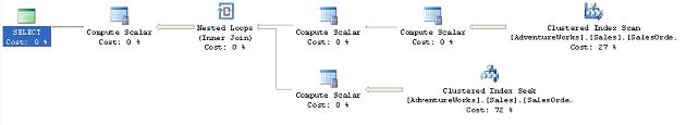
Figure 12

Instead of the Hash Match  . The loop join results in getting the first rows back very fast, but the rest of the processing was somewhat slower. So, because the plan will be concentrating on getting the first ten rows back as soon as possible, you’ll see a difference in the cost and the performance of the query. The total cost for the original query was 1.973. The hint reduced that cost to 0.012 (for the first 10 rows). The number of logical reads increases dramatically, 1238 for the un-hinted query to 101,827 for the hinted query, but the actual speed of the execution of the query increases only marginally, from around 4.2 seconds to 5 seconds. This slight slow-down in performance was accepted by the end-users since they got what they really wanted, a very fast display to the screen.

If you want to see the destructive as well as beneficial effects that hints can have, try applying the LOOP JOIN   hint, from the previous section. It increases the cost by a factor of five!

FORCE ORDER 

You’ve identified a query that is performing poorly. It’s a somewhat long query with a few tables. Normally, the optimizer will determine the order in which the joins occur but using the FORCE ORDER   hint you can make the optimizer use the order of joins as listed in the query itself. This would be done if you’ve got a fairly high degree of certainty that your join order is better than that supplied by the optimizer. The optimizer can make incorrect choices when the statistics are not up to date, when the data distribution is less than optimal or if the query has a high degree of complexity. Here is the query in question:

Based on your knowledge of the data, you’re fairly certain that you’ve put the joins in the correct order. Here is the execution plan as it exists:

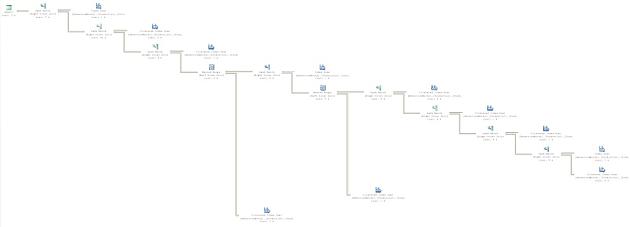
Figure   3

Obviously this is far too large to review on the page. The main point to showing the graphic is really for you to get a feel for the shape of the plan. The estimated cost as displayed in the tool tip is 0.5853.

Take the same query and apply the FORCE ORDER   query hint:

It results in the plan shown in Figure 14.

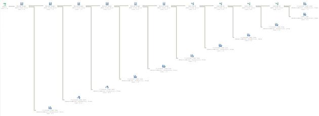
Figure   4

Don’t try to read the plan in Figure 14; simply notice that the overall shape has changed radically from the execution plan in Figure 13. All the joins are now in the exact order listed in the SELECT statement of the query. Unfortunately, our choice of order was not as efficient as the choices made by the optimizer. The estimated cost for the query displayed on the ToolTip is 1.1676. The added cost is caused by the fact that our less efficient join order is filtering less data from the early parts of the query. Instead, we’re force to carry more data between each operation.

MAXDOP 

You have one of those really nasty problems, a query that sometimes runs just fine, but sometimes runs incredibly slowly. You investigate the issue, and use SQL Server Profiler   to capture the execution of this procedure, over time, with various parameters. You finally arrive at two execution plans. The execution plan when the query runs quickly looks like this:

Figure   5

When the execution is slow, the plan looks this way (note that this image was split in order to make it more readable):

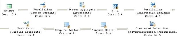
Figure   6

Here, you’re seeing a situation where the parallelism (covered in Chapter 8 of the book) that should be helping the performance of your system is, instead, hurting that performance. Since parallelism is normally turned on and off at the server level, and other procedures running on the server are benefiting from it, you can’t simply turn it off. That’s where the MAXDOP   hint becomes useful.

The MAXDOP .

In order to get this to fire on a system with only a single processor, I’m going to reset the threshold for my system as part of the query:

This will result in an execution plan that takes full advantage of parallel processing, looking like figure 16 above. The optimizer chooses a parallel execution for this plan. Look at the properties of the Clustered Index Scan   can be expanded by clicking on the plus (+) icon. It will show three different threads, the number of threads spawned by the parallel operation.

However, we know that when our query uses parallel processing, it is running slowly. We have no desire to change the overall behavior of parallelism within the server itself, so we directly affect the query that is causing problems by adding this code:

The new execution plan is limited, in this case, to a single processor, so no parallelism occurs at all. In other instances you would be limiting the degree of parallelism (e.g. two processors instead of four):

Figure   7

As you can see, limiting parallelism didn’t fundamentally change the execution plan since it’s still using a Clustered Index Scan   operator puts the data into the correct order before the Select operator adds the column aliases back in. The only real changes are the removal of the operators necessary for the parallel execution. The reason, in this instance, that the performance was worse on the production machine was due to the extra steps required to take the data from a single stream to a set of parallel streams and then bring it all back together again. While the optimizer may determine this should work better, it’s not always correct.

OPTIMIZE FOR 

You have identified a query that will run at an adequate speed for hours, or days, with no worries and then suddenly it performs horribly. With a lot of investigation and experimentation, you find that most of the time, the parameters being supplied by the application to run the procedure, result in an execution plan that performs very well. Sometimes, a certain value, or subset of values, is supplied to the parameter when the plan is recompiling and the execution plan stored in the cache with this parameter performs very badly indeed.

The OPTIMIZE FOR   hint was introduced with SQL Server 2005. It allows you to instruct the optimizer to optimize query execution for the particular parameter value that you supply, rather than for the actual value of a parameter supplied within the query.

This can be an extremely useful hint. Situations can arise whereby the data distribution of a particular table, or index, is such that most parameters will result in a good plan, but some parameters can result in a bad plan. Since plans can age out of the cache, or events can be fired that cause plan recompilation, it becomes, to a degree, a gamble as to where and when the problematic execution plan is the one that gets created and cached.

In SQL Server 2000, only two options were available:

1.  Recompile the plan every time using the RECOMPILE   hint

2. Get a good plan and keep it using the KEEPFIXED PLAN   hint

Both of these solutions (covered later in this article) could create as many problems as they solved since the RECOMPILE   hint could be applied to the problematic values as well as the useful ones.

In SQL Server 2005, when such a situation is identified that leads you to desire that one parameter be used over another, you can use the OPTIMIZE FOR   hint.

We can demonstrate the utility of this hint with a very simple set of queries:

We’ll run these at the same time and we’ll get two different execution plans:

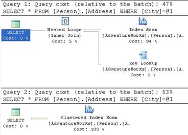
Figure   8

If you look at the cost relative to the Batch   of each of these queries, the first query is just a little less expensive than the second, with costs of 0.194 compared to 0.23. This is primarily because the second query is doing a clustered index scan, which walks through all the rows available.

If we modify our T-SQL so that we’re using parameters, like this:

We’ll get a standard execution plan for both queries that looks like this:

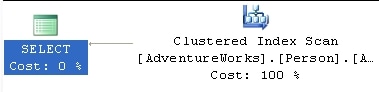
Figure   9

It’s using the clustered index for both queries now because it’s not sure which of the values available in the table is most likely going to be passed in as @City.

Let’s make one more modification. In the second query, we instruct the optimizer to optimize for Newark:

 

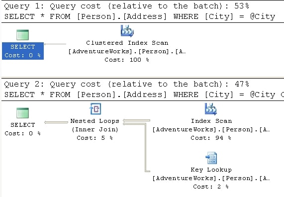
Figure 20

The value ‘London’ has very low level of selectivity   operator was able to focus the optimizer to create a plan that counted on the fact that the data was highly selective, even though it was not. The execution plan created was one for the more selective value, ‘Newark’, yet that plan helped the performance for the other value, ‘London.’

Use of this hint requires intimate knowledge of the underlying data. Choosing the wrong value to supply OPTIMIZE FOR   will not only fail to help performance, but could have a very serious negative impact. You can set as many hints as you use parameters within the query.

PARAMETERIZATION SIMPLE|FORCED 

Parameterization, forced and simple, is covered in a lot more detail in the section on Plan Guides  , in Chapter 8 of the book. It’s covered in that section because you can’t actually use this query hint by itself within a query, but must use it only with a plan guide.

RECOMPILE 

You have yet another problem query that performs slowly in an intermittent fashion. Investigation and experimentation with the query leads you to realize that the very nature of the query itself is the problem. It just so happens that this query is a built-in, ad hoc (using SQL statements or code to generate SQL statements) query of the application you support. Each time the query is passed to SQL Server, it has slightly different parameters, and possibly even a slightly different structure. So, while plans are being cached for the query, many of these plans are either useless or could even be problematic. The execution plan that works well for one set of parameter values may work horribly for another set. The parameters passed from the application in this case are highly volatile. Due to the nature of the query and the data, you don’t really want to keep all of the execution plans around. Rather than attempting to create a single perfect plan for the whole query, you identify the sections of the query that can benefit from being recompiled regularly.

The RECOMPILE   hint was introduced in SQL 2005. It instructs the optimizer to mark the plan created so that it will be discarded by the next execution of the query. This hint might be useful when the plan created, and cached, isn’t likely to be useful to any of the following calls. For example, as described above, there is a lot of ad hoc SQL in the query, or the data is relatively volatile, changing so much that no one plan will be optimal. Regardless of the cause, the determination has been made that the cost of recompiling the procedure each time it is executed is worth the time saved by that recompile.

You can also add the instruction to recompile the plan to stored procedures, when they’re created, but the RECOMPILE   query hint offers greater control. The reason for this is that statements within a query or procedure can be recompiled independently of the larger query or procedure. This means that if only a section of a query uses ad hoc SQL, you can recompile just that statement as opposed to the entire procedure. When a statement recompiles within a procedure, all local variables are initialized and the parameters used for the plan are those supplied to the procedure.

If you use local variables in your queries, the optimizer makes a guess as to what value may work best. This guess is kept in the cache. Consider the following pair of queries:

These result in an identical pair of execution plans:

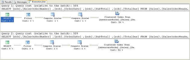
Figure 21

With a full knowledge of your system, you know that the plan for the second query should be completely different because the value passed is much more selective, and a useful index exists on that column. So, you modify the queries using the RECOMPILE   hint. In this instance, I’m adding it to both queries so that you can see that the performance gain in the second query is due to the RECOMPILE leading to a better plan, while the same RECOMPILE on the first query leads to the original plan.

This results in the following mismatched set of query plans:

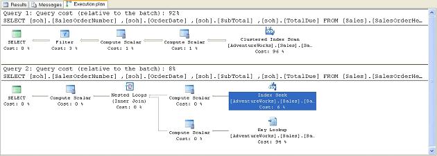
Figure 22

Note that the second query is now using our IX_SalesOrderHeader_SalesPersonID index and accounts for 8% of the combined cost of both queries, instead of 50%. This is because the Index Seek   since they will only work with a subset of the rows.

ROBUST PLAN   

This hint is used when you need to work with very wide rows. For example:

3.       A row that contains one or more variable length columns set to very large size or even the MAX size allowed in 2005

4.       A row that contains one or more large objects (LOB) such as BINARY, XML or TEXT data types.

Sometimes, when processing these rows, it’s possible for some operators to encounter errors, usually when creating worktables as part of the plan. The ROBUST PLAN  plan. This is a very rare event so this hint should only be used if you actually have a set of wide rows that cause the error condition.

KEEP PLAN 

As the data in a table changes, gets inserted or deleted, the statistics describing the data also change. As these statistics change, queries get marked for recompile. Setting the KEEP PLAN   hint doesn’t prevent recompiles, but it does cause the optimizer to use less stringent rules when determining the need for a recompile. This means that, with more volatile data, you can keep recompiles to a minimum. The hint causes the optimizer to treat temporary tables within the plan in the same way as permanent tables, reducing the number of recompiles caused by the temp table. This reduces the time and cost of recompiling a plan, which, depending on the query, can be quite large.

However, problems may arise because the old plans might not be as efficient as newer plans could be.

KEEPFIXED PLAN 

The KEEPFIXED PLAN  , but instead of simply limiting the number of recompiles, KEEPFIXED PLAN eliminates any recompile due to changes in statistics.

Use this hint with extreme caution. The whole point of letting SQL Server maintain statistics is to aid the performance of your queries. If you prevent these changed statistics from being used by optimizer, it can lead to severe performance issues.

As with KEEP PLAN,   is run against the query, forcing a recom­pile.

EXPAND VIEWS 

Your users come to you with a complaint. One of the queries they’re running isn’t returning correct data. Checking the execution plan you find that the query is running against a materialized, or indexed, view. While the performance is excellent, the view itself is only updated once a day. Over the day the data referenced by the view ages, or changes, within the table where it is actually stored. Several queries that use the view are not affected by this aging data, so changing the refresh times for the view isn’t necessary. Instead, you decide that you’d like to get directly at the data, but without completely rewriting the query.

The EXPAND VIEWS  ) clause to any indexed views within the query.

In some instances, the indexed view performs worse than the view definition. In most cases, the reverse is true. However, if the data in the indexed view is not up to date, this hint can address that issue, usually at the cost of performance. Test this hint to ensure its use doesn’t negatively impact performance.

Using one of the indexed views supplied with AdventureWorks, we can run this simple query:

Figure 23 shows the resulting execution plan:

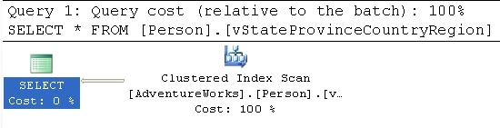
Figure 23

An indexed view is simply a clustered index, so this execution plan makes perfect sense. If we add the query hint, OPTION (EXPAND VIEWS  , things change as we see in Figure 24:

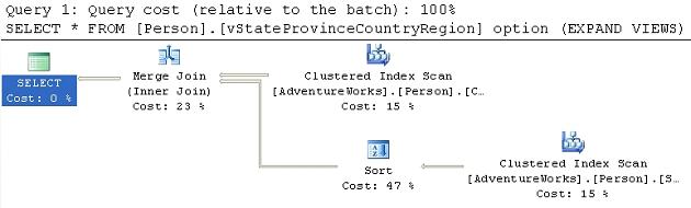
Figure 24

Now we’re no longer scanning the clustered index. Within the Optimizer, the view has been expanded into its definition so we see the Clustered Index Scan   operation. The first query has a cost estimate of .004221 as opposed to the expanded view which is estimated to cost .02848, but the data being referenced is straight from the source tables as opposed to be pulled from the clustered index that defines the materialized view.

MAXRECURSION 

With the addition of the Common Table Expression to SQL Server, a very simple method for calling recursive queries was created. The MAXRECURSION   hint places an upper limit on the number of recursions within a query.

Valid values are between 0 and 32,767. Setting the value to zero allows for infinite recursion. The default number of recursions is 100. When the number is reached, an error is returned and the recursive loop is exited. This will cause any open transactions to be rolled back. Using the option doesn’t change the execution plan but, because of the error, an actual execution plan might not be returned.

USE PLAN 

This hint simply substitutes any plan the optimizer may have created with the XML plan supplied with the hint. This is covered in great detail in Chapter 8. of the book

Join Hints 

A join hint   provides a means to force SQL Server to use one of the three join methods that we’ve encountered previously, in a given part of a query. To recap, these join methods are:

• Nested Loop ) and returns rows that satisfy the join predicate. Cost is proportional to the product of the rows in the two tables. Very efficient for smaller data sets.
• Merge join: compares two sorted inputs, one row at a time. Cost is proportional to the sum of the total number of rows. Requires an equi-join condition. Efficient for larger data sets
• Hash Match  . Does the same for the second input and then returns matching rows. Most useful for very large data sets (especially data warehouses)

By incuding one of the join hint  s in your T-SQL you will potentially override the optimizer’s choice of the most efficent join method. In general, this is not a good idea and if you’re not careful you could seriously impede performance

Application of the join hint   applies to any query (select, insert, or delete) where joins can be applied. Join hints are specified between two tables.

Consider a simple report that lists Product Models, Products and Illustrations from Adventure works:

We’ll get the following execution plan:

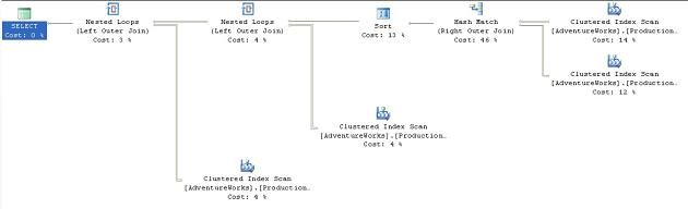
Figure 25

This is a fairly straightforward plan. The presence of the WHERE clause using the LIKE ‘%Mountain%’ condition means that there won’t be any seek on an index; and so the Clustered Index Scan   against the ProductModelIllustration table that joins to the data stream with a Loop operator. This is repeated with another Clustered Index Scan against the Illustration table and a join to the data stream with a Loop operator. The total estimated cost for these operations comes to 0.09407.

What happens if we decide that we’re smarter than the optimizer and that it really should be using a Nested Loop  ? We can force the issue by adding the LOOP hint to the join condition between Product and ProductModel:

If we execute this new query, we’ll see the following plan:

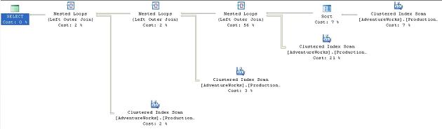
Figure 26

Sure enough, where previously we saw a Hash Match   operator. Also, the sort moved before the join in order to feed ordered data into the Loop operation, which means that the original data is sorted instead of the joined data. This adds to the overall cost. Also, note that the Nested Loop join accounts for 56% of the cost, whereas the original Hash Match accounted for only 46%. All this resulted in a total, higher cost of 0.16234.

If you replace the previous LOOP hint with the MERGE hint, you’ll see the following plan:

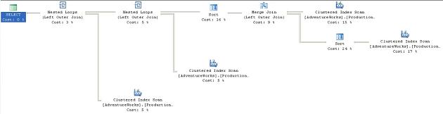
Figure 27

The Nested Loop   operator and the overall cost of the plan drops to 0.07647, apparently offering us a performance benefit.

The Merge Join  .

In order to verify the possibility of a performance increase, we can change the query options so that it shows us the I/O costs of each query. The output of all three queries is listed, in part, here:

Original (Hash)
Table ‘Illustration’. Scan count 1, logical reads 273
Table ‘ProductModelIllustration’. Scan count 1, logical reads 183
Table ‘Worktable’. Scan count 0, logical reads 0
Table ‘ProductModel’. Scan count 1, logical reads 14
Table ‘Product’. Scan count 1, logical reads 15

Loop
Table ‘Illustration’. Scan count 1, logical reads 273
Table ‘ProductModelIllustration’. Scan count 1, logical reads 183
Table ‘Product’. Scan count 1, logical reads 555
Table ‘ProductModel’. Scan count 1, logical reads 14

Merge
Table ‘Illustration’. Scan count 1, logical reads 273
Table ‘ProductModelIllustration’. Scan count 1, logical reads 183
Table ‘Product’. Scan count 1, logical reads 15
Table ‘ProductModel’. Scan count 1, logical reads 14

This shows us that the Merge and Loop joins required almost exactly the same number of reads to arrive at the data set needed as the original Hash join. The differences come when we see that, in order to support the Loop join, 555 reads were required instead of 15 for both the Merge and Hash joins. The other difference, probably the clincher in this case, is the work table that the Hash creates to support the query. This was eliminated with the Merge join. This illustrates the point that the optimizer does not always choose an optimal plan. Based on the statistics in the index and the amount of time it had to calculate its results, it must have decided that the Hash join would perform faster. In fact, as the data changes within the tables, it’s possible that the Merge join will cease to function better over time, but because we’ve hard coded the join, no new plan will be generated by the optimizer as the data changes, as would normally be the case.

Table Hints 

Table hints enable you to specifically control how the optimizer “uses” a particular table when generating an execution plan. For example, you can force the use of a table scan, or specify a particular index that you want used on that table.

As with the query and join hint  s, using a table hint circumvents the normal optimizer processes and could lead to serious performance issues. Further, since table hints can affect locking strategies, they possibly affect data integrity leading to incorrect or lost data. These must be used judiciously.

Some of the table hints are primarily concerned with locking strategies. Since some of these don’t affect execution plans, we won’t be covering them. The three table hints covered below have a direct impact on the execution plans. For a full list of table hints, please refer to the Books Online supplied with SQL Server 2005.

Table Hint Syntax 

The correct syntax in SQL Server 2005 is to use the WITH keyword and list the hints within a set of parenthesis like this:

The WITH keyword is not required in all cases, nor are the commas required in all cases, but rather than attempt to guess or remember which hints are the exceptions, all hints can be placed within the WITH clause and separated by commas as a best practice to ensure consistent behavior and future compatibility. Even with the hints that don’t require the WITH keyword, it must be supplied if more than one hint is to be applied to a given table.

NOEXPAND 

When multiple indexed views are referenced within the query, use of the NOEXPAND  into its underlying view definition. This allows for a more granular control over which of the indexed views is forced to resolve to its base tables and which simply pull their data from the clustered index that defines it.

SQL 2005 Enterprise and Developer editions will use the indexes in an indexed view if the optimizer determines that index will be best for the query. This is called indexed view matching. It requires the following settings for the connection:

• ANSI_NULL set to on
• ANSI_WARNINGS set to on
• CONCAT_NULL_YIELDS_NULL set to on
• ANSI_PADDING set to on
• ARITHABORT set to on
• QUOTED_IDENTIFIERS set to on
• NUMERIC_ROUNDABORT set to off

Using the NOEXPAND  , vStateProvinceCountryRegion, in AdventureWorks. The optimizer expanded the view and we saw an execution plan that featured a 3-table join. We change that behavior using the NOEXPAND hint

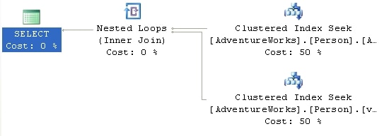
Figure 28

Now, not only are we using the clustered index defined on the view, but we’re seeing a performance increase, with the estimated cost decreasing from .00985 to .00657.

INDEX() 

The index() table hint allows you to define the index to be used when accessing the table. The syntax supports either numbering the index, starting at 0 with the clustered index, if any, and proceeding one at a time through the rest of the indexes:

However, I recommend that you simply refer to the index by name because the order in which indexes are applied to a table can change (although the clustered index will always be 0):

You can only have a single index hint for a given table, but you can define multiple indexes within that one hint.

Let’s take a simple query that lists Department Name, Title and Employee Name:

We get a standard execution plan:

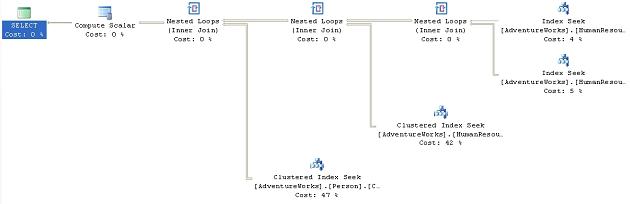
Figure 29

We see a series of Index Seek   operations. Suppose we’re convinced that we can get better performance if we could eliminate the Index Seek on the HumanResources.Department table and instead use that table’s clustered index, PK_Department_DepartmentID. We could accomplish this using the INDEX hint, as follows:

This results in the following execution plan:

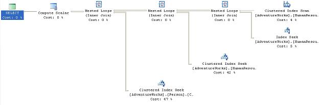
Figure 30

We can see the Clustered Index Scan  . This change causes a marginally more expensive query, with the cost coming in at 0.0739643 as opposed to 0.0739389. While the index seek is certainly faster than the scan, the difference at this time is small because the scan is only hitting a few more rows than the seek, in such a small table. However, using the clustered index didn’t improve the performance of the query as we originally surmised because the query used it within a scan instead of the more efficient seek operation.

FASTFIRSTROW   

Just like the FAST n   forces the optimizer to choose a plan that will return the first row as fast as possible for the table in question. Functionally, FASTFIRSTROW is equivalent to the FAST n query hint, but it is more granular in its application.

Microsoft recommends against using FASTFIRSTROW   as it may be removed in future versions of SQL Server. Nevertheless, we’ll provide a simple example. The following query is meant to get a summation of the available inventory by product model name and product name:

It results in this execution plan:

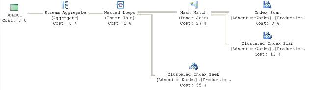
Figure 31

As you can see, an Index Scan   operator.

If we decided that we thought that getting the Product information a bit quicker might make a difference in the behavior of the query we could add the table hint, only to that table:

This gives us the following execution plan:

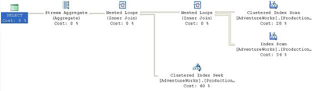
Figure 32

This makes the optimizer choose a different path through the data. Instead of hitting the ProductModel table first, it’s now collecting the Product information first. This is being passed to a Nested Loop   operator that will loop through the smaller set of rows from the Product table and compare them to the larger data set from the ProductModel table.

The rest of the plan is the same. The net result is that, rather than building the worktable to support the hash match join, most of the work occurs in accessing the data through the index scans and seeks, with cheap nested loop joins replacing the hash join  s. The cost estimate decreases from .101607 in the original query to .011989 in the second.

One thing to keep in mind, though, is that while the performance win seems worth it in this query, it comes at the cost of a change in the scans against the ProductModel table. Instead of one scan and two reads, the second query has 504 scans and 1008 reads against the ProductModel table. This appears to be less costly than creating the worktable, but you need to remember these tests are being run against a server in isolation. I’m running no other database applications or queries against my system at this time. That kind of additional I/O could cause this process, which does currently run faster ~130ms vs. ~200ms, to slow down significantly.

Summary

While the Optimizer makes very good decisions most of the time, at times it may make less than optimal choices. Taking control of the queries using Table, Join and Query hints where appropriate can be the right choice. Remember that the data in your database is constantly changing. Any choices you force on the Optimizer through these hints today to achieve whatever improvement you’re hoping for may become a major pain in your future. Test the hints prior to applying them and remember to document their use in some manner so that you can come back and test them again periodically as your database grows. As Microsoft releases patches and service packs, behavior of the optimizer can change. Be sure to retest any queries using hints after an upgrade to your server. I intentionally found about as many instances where the query hints would help and where the query hints hurt to put the point across; use of these hints should be considered as a last resort, not a standard method of operation.